Introduction to Statistics for the Social Sciences SBS

Introduction to Statistics for the Social Sciences SBS 200, COMM 200, GEOG 200, PA 200, POL 200, or SOC 200 Lecture Section 001, Spring 2015 Room 150 Harvill Building 8: 00 - 8: 50 Mondays, Wednesdays & Fridays.

Labs continue this week with Project 2 presentations
 Please read chapters 10")
Schedule of readings Before next exam (Monday May 4 th) Please read chapters 10 – 14 Please read Chapters 17, and 18 in Plous Chapter 17: Social Influences Chapter 18: Group Judgments and Decisions
 Homework due – Monday (April 20")
No homework due – Friday (April 17 th) Homework due – Monday (April 20 th) On class website: Please print and complete homeworksheet #19 Completing Simple Regression using Excel

Use this as your study guide Next couple of lectures 4/15/15 Logic of hypothesis testing with Correlations Interpreting the Correlations and scatterplots Simple and Multiple Regression

+0. 9199 3 0. 878
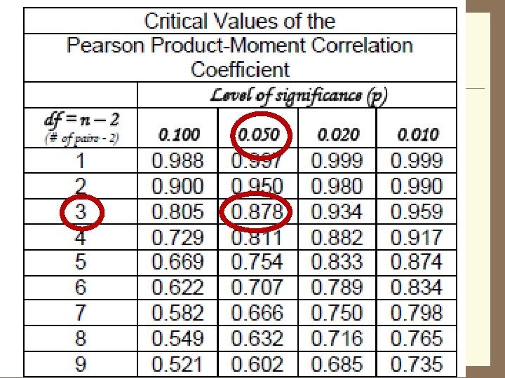

+0. 9199 3 0. 878 Yes The relationship between the hours worked and weekly pay is a strong positive correlation. This correlation issignificant, r(3) = 0. 92; p < 0. 05

3 -0. 73 3 0. 878 No No The relationship between wait time and number of operators working is negative and strong, but not reliable enough to reach significance. This correlation isnot significant, r(3) = -0. 73 ; n. s.

We are measuring 9 students
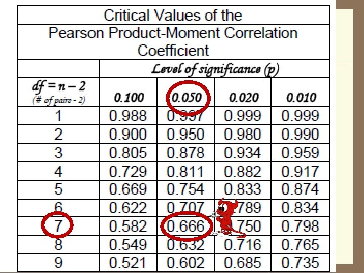

4. 0 3. 0 2. 0 1. 0 GPA 4. 0 GPA Critical r = 0. 666 2. 0 1. 0 0 1 2 3 4 High School GPA r(7) = 0. 50 ct Null Reje ificant ign r is s r(7) = + 0. 911444123 2. 0 1. 0 0 200 300 400 500 600 SAT (Verbal) ull n t c e t rej ificant r(7) =o +no 0. 80 D ign s t o r is n r(7) = + 0. 616334867 0 200 300 400 500 600 SAT (Mathematical) ull n t c reje icant t o n r(7) nif Do = + t 0. 80 g i s o r is n r(7) = + 0. 487295007

4. 0 3. 0 2. 0 1. 0 GPA 4. 0 2. 0 1. 0 0 1 2 3 4 High School GPA 2. 0 1. 0 0 200 300 400 500 600 SAT (Verbal) 0 200 300 400 500 600 SAT (Mathematical) r(7) = 0. 50 r(7) = + 0. 80 r(7) = + 0. 911444123 r(7) = + 0. 616334867 r(7) = + 0. 487295007

4. 0 3. 0 2. 0 1. 0 GPA 4. 0 2. 0 1. 0 0 1 2 3 4 High School GPA 2. 0 1. 0 0 200 300 400 500 600 SAT (Verbal) 0 200 300 400 500 600 SAT (Mathematical) r(7) = 0. 50 r(7) = + 0. 80 r(7) = + 0. 911444123 r(7) = + 0. 616334867 r(7) = + 0. 487295007

4. 0 3. 0 2. 0 1. 0 GPA 4. 0 2. 0 1. 0 0 1 2 3 4 High School GPA 2. 0 1. 0 0 200 300 400 500 600 SAT (Verbal) 0 200 300 400 500 600 SAT (Mathematical) r(7) = 0. 50 r(7) = + 0. 80 r(7) = + 0. 911444123 r(7) = + 0. 616334867 r(7) = + 0. 487295007

Correlation: Independent and dependent variables • When used for prediction we refer to the predicted variable as the dependent variable and the predictor variable as the independent variable What are we predicting? Dependent Variable Independent Variable Dependent Variable What are we predicting? Independent Variable

Correlation - What do we need to define a line If you probably make this much Yearly Income Y-intercept = “a” (also “b 0”) Where the line crosses the Y axis Slope = “b” (also “b 1”) How steep the line is Expenses per year If you spend this much • The predicted variable goes on the “Y” axis and is called the dependent variable • The predictor variable goes on the “X” axis and is called the independent variable

Angelina Jolie Buys Brad Pitt a $24 million Heart-Shaped Island for his 50 th Birthday Yearly Income Angelina probably makes this much Dustin probably makes this much Expenses Dustin spent per year this much Angelina spent this much Dustin spends $12 for his Birthday Revisit this slide

Assumptions Underlying Linear Regression • For each value of X, there is a group of Y values • • These Y values are normally distributed. The means of these normal distributions of Y values all lie on the straight line of regression. • The standard deviations of these normal distributions are equal.

Correlation - the prediction line - what is it good for? Prediction line • makes the relationship easier to see (even if specific observations - dots - are removed) • identifies the center of the cluster of (paired) observations • identifies the central tendency of the relationship (kind of like a mean) • can be used for prediction • should be drawn to provide a “best fit” for the data • should be drawn to provide maximum predictive power for the data • should be drawn to provide minimum predictive error

- Slides: 22