Introduction to Statistics for the Social Sciences SBS

Introduction to Statistics for the Social Sciences SBS 200 - Lecture Section 001, Fall 2017 Room 150 Harvill Building 10: 00 - 10: 50 Mondays, Wednesdays & Fridays.

Screen Lecturer’s desk Row A Row B Row A 15 14 12 11 10 13 20 Row B 19 24 23 22 21 Row C 20 19 28 27 26 25 24 23 Row D 22 21 20 19 30 29 28 27 26 25 24 23 Row E 23 22 21 20 19 35 34 33 32 31 30 29 28 27 26 Row F 25 35 34 33 32 31 30 29 28 27 26 Row G 37 36 35 34 33 32 31 30 29 28 41 40 39 38 37 36 35 34 33 32 31 30 Row C Row D Row E Row F Row G Row H Row L 33 31 29 25 23 22 21 21 8 7 6 5 3 4 Row A 2 1 3 2 Row B 9 8 7 6 5 4 12 11 10 9 8 7 6 5 4 3 2 1 24 23 22 21 20 19 18 17 16 15 14 13 12 11 10 9 8 7 6 5 4 3 2 1 Row F 25 24 23 22 21 20 19 18 17 16 15 14 13 12 11 10 9 8 7 6 5 4 3 2 1 Row G Row H 27 26 25 24 23 22 21 20 19 18 17 16 15 14 13 12 29 Row J 28 27 26 25 24 23 22 21 20 19 18 17 16 15 14 13 12 11 10 9 8 7 6 5 4 3 2 1 Row J 29 Row K 28 27 26 25 24 23 22 21 20 19 18 17 16 15 14 13 12 11 10 9 8 7 6 5 4 3 2 1 Row K 25 Row L 24 23 22 21 20 19 18 17 16 15 14 13 12 11 10 9 20 19 Row M 18 4 3 Row N 15 14 13 12 11 10 9 8 7 6 5 4 3 2 1 Row P 15 14 13 12 11 10 9 8 7 6 5 4 3 2 1 4 3 32 31 30 29 28 27 26 Row M 9 18 17 18 16 17 15 16 18 14 15 17 18 13 14 13 16 17 12 11 10 15 16 14 15 13 12 11 10 14 17 16 15 14 13 12 11 10 9 13 8 7 6 5 table 15 14 13 12 11 10 9 8 7 6 Projection Booth 5 2 1 1 1 Row C Row D Row E 11 10 9 8 7 6 5 4 3 2 2 1 1 1 Row L Row M Harvill 150 renumbered Left handed desk Row H

A note on doodling

Everyone will want to be enrolled in one of the lab sessions Continue Project 3 This Week
 Please read chapters 1 -")
Schedule of readings Before next exam (November 17 th) Please read chapters 1 - 11 in Open. Stax textbook Please read Chapters 2, 3, and 4 in Plous Chapter 2: Cognitive Dissonance Chapter 3: Memory and Hindsight Bias Chapter 4: Context Dependence

. … s me a n k c Sum i n r g o De of S n f i s a l q U g u u r : ares e ? m n e r e o s i o c of fr t f SS n s a s i e i r eedo a Qu what v E m df L P M A S “SS” = “Sum of Squares” “SS”= =degrees “Sum ofof. Squares” “df” freedom Remember, you should know these four formulas by heart We lose one degree of freedom for every parameter we estimate

… e c n a i r a v e l r p o m f a a s l u r u ? m o r e o c is f n a s s i i i SS r a Th what v E L P d f M A S ANOVA table Source Between Within Total SS df MS F 40 88 128 ? ? ? ?

Writing Assignment - ANOVA 1. Write formula for standard deviation of sample 2. Write formula for variance of sample 3. Re-write formula for variance of sample using the nicknames for the numerator and denominator 4. Complete this ANOVA table 5. Given a critical F(2, 12) = 3. 89 Write a summary statement of findings (all three parts) SS = MS df ANOVA table Source Between Within Total SS df MS F 40 88 128 ? ? ? ? ux d Re

“SS” = “Sum of Squares” - will be given for exams Source Between Within Total ANOVA table SS df 40 ? 88 ? ? 128 ? 2 ? 14 F MS # groups - 1 ? ? 3 -1=2 ? 15 -3=12 # scores - number of groups # scores - 1 15 - 1=14 ux d Re

ANOVA table 40 SSbetween 2 ANOVA table dfbetween “SS” = “Sum of Squares” - will be given for exams Source Between Within Total SS df 40 88 128 2 12 14 88 12 MS 20 ? ? 7. 33 SSwithin dfwithin 40 =20 2 F ? 2. 73 MSbetween MSwithin 20 =2. 73 7. 33 88 =7. 33 12 ux d Re

Make decision whether or not to reject null hypothesis Observed F = 2. 73 Critical F(2, 12) = 3. 89 2. 73 is not farther out on the curve than 3. 89 so, we do not reject the null hypothesis F(2, 12) = 2. 73; n. s. Conclusion: There appears to be no main effect of type of incentive on number of girl scout cookies sold The average number of cookies sold for three different incentives were compared. The mean number of cookie boxes sold for the “Hawaii” incentive was 14 , the mean number of cookies boxes sold for the “Bicycle” incentive was 12, and the mean number of cookies sold for the “No” incentive was 10. An ANOVA was conducted and there appears to be no main effect of the number of cookies sold as a result of the different levels of incentive F(2, 12) = 2. 73; n. s. ux d Re

ur o y d in n a H ing writ a ent m n ssig

Main effect of incentive: Will offering an incentive result in more girl scout cookies being sold? If we have a “effect” of incentive then the means are significantly different from each other • we reject the null • we have a significant F • p < 0. 05 We don’t know which means are different from which …. just that they are not all the same To get an effect we want: • Large “F” - big effect and small variability • Small “p” - less than 0. 05 (whatever our alpha is)

Let’s do same problem Using MS Excel A girlscout troop leader wondered whether providing an incentive to whomever sold the most girlscout cookies would have an effect on the number cookies sold. She provided a big incentive to one troop (trip to Hawaii), a lesser incentive to a second troop (bicycle), and no incentive to a third group, and then looked to see who sold more cookies. Troop 1 (Nada) 10 8 12 7 13 Troop 2 (bicycle) 12 14 10 11 13 Troop 3 (Hawaii) 14 9 19 13 15 n=5 x = 10 n=5 x = 12 n=5 x = 14
")
Let’s do one Replication of study (new data)

Let’s do same problem Using MS Excel

Let’s do same problem Using MS Excel

ANOVA table “Sum of Squares” SSbetween 40 =20 2 dfbetween # groups - 1 20 =2. 73 7. 33 3 -1=2 # scores - # of groups 15 -3=12 # scores - 1 15 - 1=14 MSbetween MSwithin SSwithin dfwithin 88 =7. 33 12

No, so it is not significant Do not reject null “Sum of Squares” F critical P-value (is it less than. 05? ) (is observed F greater than critical F? )

Make decision whether or not to reject null hypothesis Observed F = 2. 73 Critical F(2, 12) = 3. 89 2. 7 is not farther out on the curve than 3. 89 so, we do not reject the null hypothesis Also p-value is not smaller than 0. 05 so we do not reject the null hypothesis Step 6: Conclusion: There appears to be no effect of type of incentive on number of girl scout cookies sold

Make decision whether or not to reject null hypothesis Observed F = 2. 7272 Critical F(2, 12) = 3. 88529 F(2, 12) = 2. 73; n. s. 2. 7 is not farther out on the curve than 3. 89 so, we do not reject the null hypothesis Conclusion: There appears to be no effect of type of incentive on number of girl scout cookies sold The average number of cookies sold for three different incentives were compared. The mean number of cookie boxes sold for the “Hawaii” incentive was 14 , the mean number of cookies boxes sold for the “Bicycle” incentive was 12, and the mean number of cookies sold for the “No” incentive was 10. An ANOVA was conducted and there appears to be no significant difference in the number of cookies sold as a result of the different levels of incentive F(2, 12) = 2. 73; n. s.

Homework

Homework

Homework

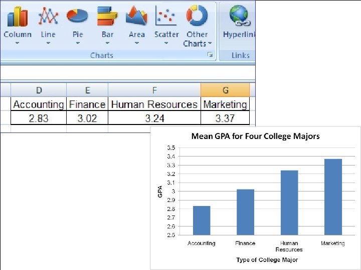
Type of major in school 4 (accounting, finance, hr, marketin Homework Grade Point Average 0. 05 2. 83 3. 02 3. 24 3. 37

If observed F is bigger than critical F: F: If observed F is bigger critical Reject null & Significant! Homework If p value is less than 0. 05: Reject null & Significant! 4 -1=3 # groups - 1 # scores - number of groups 28 - 4=24 # scores - 1 28 - 1=27 0. 3937 0. 1119 0. 3937 / 0. 1119 = 3. 517 3. 009 3 24 0. 03
 = 3. 517; p < 0. 05 The GPA")
Yes Homework F (3, 24) = 3. 517; p < 0. 05 The GPA for four majors was compared. The average GPA was 2. 83 for accounting, 3. 02 for finance, 3. 24 for HR, and 3. 37 for marketing. An ANOVA was conducted and there is a significant difference in GPA for these four groups (F(3, 24) = 3. 52; p < 0. 05).

Number of observations in each group Average for each group (We REALLY care about this one)

“SS” = “Sum of Squares” - will be given for exams Number of groups minus one (k – 1) 4 -1=3 Number of people minus number of groups (n – k) 28 -4=24

SS between df between SS within df within MS between MS within
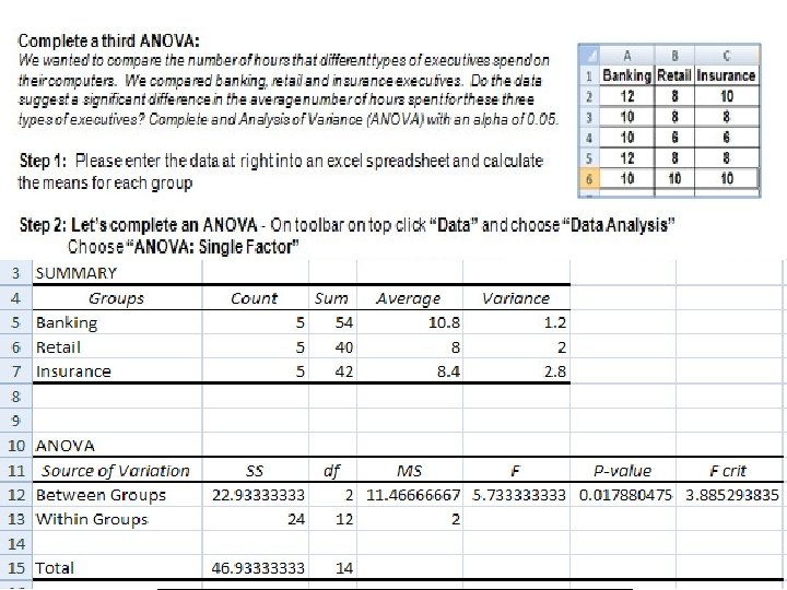
 Hours spent at computer 0. 05 10.")
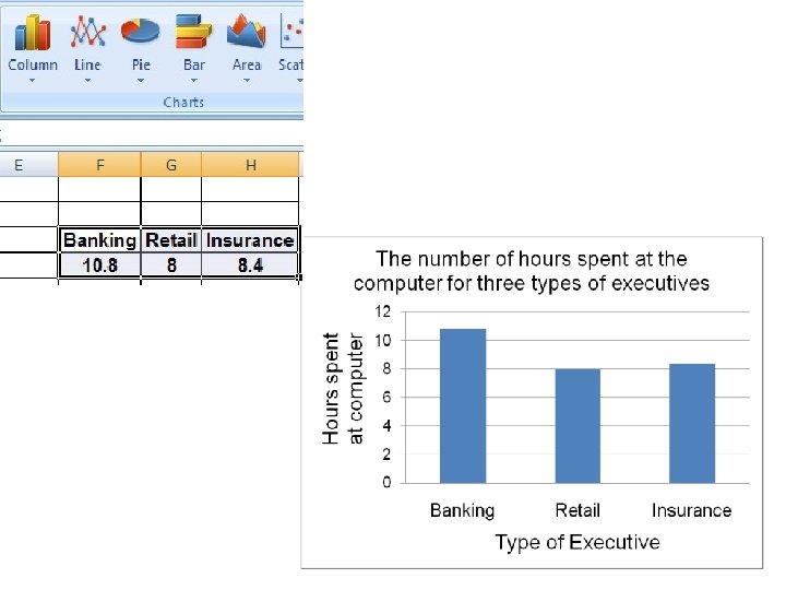
Type of executive 3 (banking, retail, insurance) Hours spent at computer 0. 05 10. 8 8 8. 4

If observed F is bigger than critical F: F: If observed F is bigger than critical Reject null & Significant! If p value is less than 0. 05: Reject null & Significant! 11. 46 2 11. 46 / 2 = 5. 733 3. 88 2 12 0. 0179
 = 5. 73; p < 0. 05 The number of")
Yes F (2, 12) = 5. 73; p < 0. 05 The number of hours spent at the computer was compared for three types of executives. The average hours spent was 10. 8 for banking executives, 8 for retail executives, and 8. 4 for insurance executives. An ANOVA was conducted and we found a significant difference in the average number of hours spent at the computer for these three groups , (F(2, 12) = 5. 73; p < 0. 05).

Number of observations in each group Average for each group Just add up all scores

“SS” = “Sum of Squares” - will be given for exams Number of groups minus one (k – 1) 3 -1=2 Number of people minus number of groups (n – k) 15 -3=12

SS between df between SS within df within MS between MS within
")
. “Between Groups” Difference Variability between means “Within Groups” Variability of curve(s)

One way analysis of variance Variance is divided Remember, one-way = one IV Total variability Between group variability (only one factor) Remember, 1 factor = 1 independent variable (this will be our numerator – like difference between means) Within group variability (error variance) Remember, error variance = random error (this will be our denominator – like within group variability
 Describe the")
Five steps to hypothesis testing Step 1: Identify the research problem (hypothesis) Describe the null and alternative hypotheses Step 2: Decision rule • Alpha level? (α =. 05 or. 01)? Still, difference • Critical statistic (e. g. z or t or F or r) value? between means Step 3: Calculations F= MSBetween MSWithin Step 4: Make decision whether or not to reject null hypothesis Still, variability If observed t (or F) is bigger then critical t (or F) then of curve(s) reject null Step 5: Conclusion - tie findings back in to research problem
: The sum of squared deviations of some set of scores")
Sum of squares (SS): The sum of squared deviations of some set of scores about their mean Mean squares (MS): The sum of squares divided by its degrees of freedom Mean square between groups: sum of squares between groups divided by its degrees of freedom Mean square total: sum of squares total divided by its degrees of freedom Mean square within groups: sum of squares within groups divided by its degrees of freedom F= MSBetween MSWithin

ANOVA F= Variability between groups Variability within groups Variability Between Groups “Between” variability bigger than “within” variability so should get a big (significant) F Variability Within Groups Variability Between Groups “Between” variability getting smaller “within” variability staying same so, should get a smaller F Variability Within Groups Variability Between Groups “Between” variability getting very small “within” variability staying same so, should get a very small F Variability Within Groups

ANOVA F= Variability between groups Variability within groups Variability Between Groups “Between” variability bigger than “within” variability so should get a big (significant) F Variability Within Groups Variability Between Groups “Between” variability getting smaller “within” variability staying same so, should get a smaller F Variability Within Groups “Between” variability getting very small “within” variability staying same so, should get a very small F (equal to 1)

Let’s try one In a one-way ANOVA we have three types of variability. Which picture best depicts the random error variability (also known as the within variability)? a. Figure 1 b. Figure 2 1. c. Figure 3 correct d. All of the above 2. 3.

Let’s try one In a one-way ANOVA we have three types of variability. Which picture best depicts the between group variability? a. Figure 1 b. Figure 2 correct c. Figure 3 1. d. All of the above 2. 3.

QUESTIONS?

- Slides: 51