Introduction to Statistics for the Social Sciences SBS

Introduction to Statistics for the Social Sciences SBS 200 - Lecture Section 001, Fall 2019 Social Sciences Room 100 10: 00 - 10: 50 Mondays, Wednesdays & Fridays. November 4

A note on doodling
 Please read chapters 1 - 11")
Schedule of readings Before next exam (November 22) Please read chapters 1 - 11 in Open. Stax textbook Please read Chapters 2, 3, and 4 in Plous Chapter 2: Cognitive Dissonance Chapter 3: Memory and Hindsight Bias Chapter 4: Context Dependence

Labs continue this week
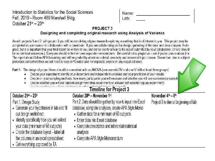

This lab builds on the work we did in our very first lab. But now we are using the correlation for prediction. This is called regression analysis 4 Project lations e r r o C ses y l a - Two n A ssion e r g e R - Two
 and the predictor")
We refer to the predicted variable as the dependent variable (Y) and the predictor variable (X) as the independent variable Why are we finding the regression line? How would we use it? ion s s re ent g e r ici e) f f coe (slop corr e coef lation ficie (“r”) nt
 b. Age")
What variable are we predicting? a. Height of Boys in 1990 (cm) b. Age of boys in 1990 c. Both height and age of boys in 1990

If a boy is 8 -years old how tall would we predict he would be? Complete prediction “by eye” looking at graph? a. 40 cm b. 80 cm c. 120 cm math e h t o d let’s n u f d. 160 cm r o f t 76 = 122 us J 4. 4 6 + ) 8 ( 21 Y’ = 7. 15

If a boy is 2 -years old how tall would we predict he would be? Complete prediction “by eye” looking at graph? a. 40 cm b. 80 cm c. 120 cm math e h t o d let’s n u f d. 160 cm 8. 8 r o f t Jus. 476 = 7 + 64 ) 2 ( 1 2 Y’ = 7. 15
 b. Number of")
What variable are we predicting? a. Size of state (square miles) b. Number of letters in name of state c. Both size of state and number of letters
 how large would")
If a state has 7 letters in the name (like Arizona) how large would we predict the state to be? Complete prediction “by eye” looking at graph? a. 20, 000 square miles b. 30, 000 square miles c. 40, 000 square miles math e h t o d let’s 53 n u f d. 50, 000 square miles r o f t 4 = 49, 9 us J 67, 88 + ) 7 ( 61. 5 5 , 2 = ’ Y
 b. Sales price of")
What variable are we predicting? a. Size of TV (inches) b. Sales price of TV ($) c. Both sales price and size of TV

If a TV is 55 inches what would we predict cost to? Complete prediction “by eye” looking at graph? a. $1, 500 b. $1, 725 c. $2, 000 math e h t o d let’s 35 n u d. $2, 225 f r o f st 5 = $2, 2 Ju 2. 2 6 7 – ) 5 44 (5 0. 5 5 = ’ Y

If a TV is 40 inches what would we predict cost to? Complete prediction “by eye” looking at graph? a. $1, 500 b. $1, 725 c. $2, 000 math e h t o d let’s 9 n u d. $2, 225 f r o f 5 = $1, 43 st Ju 62. 2 7 – ) 0 4 44 ( 0. 5 5 = ’ Y

What variable are we predicting? a. Amount of Wine Consumed b. Death Rate in the Country c. Both Amount of Wine Consumed and Death Rate
 what would we")
If a country consumes an average of 8 liters (per capita) what would we predict death rate from heart disease be? Complete prediction “by eye” looking at graph? a. 50 b. 75 math e h t o c. 100 d let’s n u f 5. 6 7 r o = f 3 t s 6 u. J d. 125 ) + 266 . 878 Y’ = -23 (8

Review of Quiz from Friday as a warm-up p r grou e p 1 n or 1. When do you use a t-test and when do you use an ANOVA or n-2 groups # of n l a Tot s n a e m 2. What is the formula of freedom in a two-sample t-test e twofor rdegrees r a p e m mo s co t-test A compares s degrees of freedom “between groups” in ANOVA 3. What the formula ANis. OV meanfor o w t than ps - 1 u o r g of 4. What is the formula for degrees of#freedom “within groups” in ANOVA roup g r e p 5. How are “levels”, “groups”, “conditions” “treatments” related? n -1 or roups g f o n-# ean effect” l m a l t l 6. How are “significant difference”, “p< 0. 05”, “main o a T They ing and “we reject the null” related? the same th l mean l a y e 7. Draw and Th matchteach hing with proper label e m a the s oup r G p u n o i r With ween G t l e a B t o iability T y r t i a l i V b a i ility Variab

Review of Quiz from Friday as a warm-up 8. Daphne compared running speed for three types of running of Typeas shoes. She asked 10 people to run as fast they could g n i n run 30 people altogether g type of shoe. So, there wearing one n i n n u R shoe d e • What is the independent variable? e Sp • What is the dependent variable? Type 1 • How many factors do we have (what are they)? Type 2 3 Type 3 s p • How many treatments do we have (what are they)? u r gro Facto 1 9. Complete this ANOVA table SSB df. B # groups - 1 n - # groups n-1 SSW df. W Yes 10. Find the critical F value from the table F(2, 27)=4. 00; p< 0. 05 MSB MSW 3. 37 11. Is there a main effect of type of running shoe? Is “p< 0. 05”?

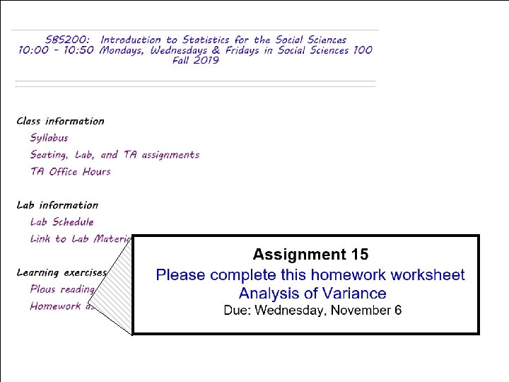
Complete worksheet for next class

Complete worksheet for next class

Complete worksheet for next class

- Slides: 27