Introduction to Statistics for the Social Sciences SBS

Introduction to Statistics for the Social Sciences SBS 200, COMM 200, GEOG 200, PA 200, POL 200, or SOC 200 Lecture Section 001, Fall 2015 Room 150 Harvill Building 10: 00 - 10: 50 Mondays, Wednesdays & Fridays. http: //courses. eller. arizona. edu/mgmt/delaney/d 15 s_database_weekone_screenshot. xlsx

By the end of lecture today 11/9/15 Analysis of Variance (ANOVA) The ANOVA table

Before next exam (November 20 th) Please read chapters 1 – 11 + 13 in Open. Stax textbook Please read Chapters 2, 3, and 4 in Plous Chapter 2: Cognitive Dissonance Chapter 3: Memory and Hindsight Bias Chapter 4: Context Dependence

Homework Assignment Go to D 2 L - Click on “Interactive Online Homework Assignments” Complete Assignment 20: HW 18 -Hypothesis testing, Analysis of Variance (ANOVA) Using Excel Due: Friday, November 13 th

Everyone will want to be enrolled in one of the lab sessions No Labs this week No Class On Wednesday

Five steps to hypothesis testing Step 1: Identify the research problem (hypothesis) Describe the null and alternative hypotheses Step 2: Decision rule • Alpha level? (α =. 05 or. 01)? Still, difference • Critical statistic (e. g. z or t or F or r) value? between means Step 3: Calculations F= MSBetween MSWithin Step 4: Make decision whether or not to reject null hypothesis Still, variability If observed t (or F) is bigger then critical t (or F) then of curve(s) reject null Step 5: Conclusion - tie findings back in to research problem

. “Between Groups” Difference Variability between means “Within Groups” Variability of curve(s)

Sum of squares (SS): The sum of squared deviations of some set of scores about their mean Mean squares (MS): The sum of squares divided by its degrees of freedom Mean square between groups: sum of squares between groups divided by its degrees of freedom Mean square total: sum of squares total divided by its degrees of freedom Mean square within groups: sum of squares within groups divided by its degrees of freedom F= MSBetween MSWithin

One way analysis of variance Variance is divided Remember, one-way = one IV Total variability Between group variability (only one factor) Remember, 1 factor = 1 independent variable (this will be our numerator – like difference between means) Within group variability (error variance) Remember, error variance = random error (this will be our denominator – like within group variability

ANOVA F= Variability between groups Variability within groups Variability Between Groups “Between” variability bigger than “within” variability so should get a big (significant) F Variability Within Groups Variability Between Groups “Between” variability getting smaller “within” variability staying same so, should get a smaller F Variability Within Groups Variability Between Groups “Between” variability getting very small “within” variability staying same so, should get a very small F Variability Within Groups

ANOVA F= Variability between groups Variability within groups Variability Between Groups “Between” variability bigger than “within” variability so should get a big (significant) F Variability Within Groups Variability Between Groups “Between” variability getting smaller “within” variability staying same so, should get a smaller F Variability Within Groups “Between” variability getting very small “within” variability staying same so, should get a very small F (equal to 1)

. Effect size is considered relative to variability of distributions Treatment Effect x Variability between groups Variability within groups Treatment Effect x

One-way ANOVA versus Chi Square Be careful you are not designing a Chi Square If this is just frequency you may have a problem Total Number of Boxes Sold Sales per Girl scout This is an ANOVA This is a Chi Square None New Bike These are means Trip Hawaii New Trip Bike Hawaii These are just frequencies None

Let’s try one In a one-way ANOVA we have three types of variability. Which picture best depicts the random error variability (also known as the within variability)? a. Figure 1 b. Figure 2 1. c. Figure 3 d. All of the above 2. 3.

Let’s try one In a one-way ANOVA we have three types of variability. Which picture best depicts the between group variability? a. Figure 1 b. Figure 2 c. Figure 3 1. d. All of the above 2. 3.

Let’s try one F= Variability between groups Variability within groups Which figure would depict the largest F ratio a. Figure 1 b. Figure 2 c. Figure 3 d. All of the above 1. 2. 3. “F ratio” is referring to "observed F”

If your observed z is within one standard deviation of the mean, you will never reject the null Let’s try one Winnie found an observed z of. 74, what should she conclude? (Hint: notice that. 74 is less than 1) a. Reject the null hypothesis b. Do not reject the null hypothesis c. Not enough info is given x x small observed z score

Let’s try one Winnie found an observed t of. 04, what should she conclude? (Hint: notice that. 04 is less than 1) a. Reject the null hypothesis b. Do not reject the null hypothesis c. Not enough info is given x small observed t score

Let’s try one Winnie found an observed F ratio of. 9, what should she conclude? a. Reject the null hypothesis b. Do not reject the null hypothesis c. Not enough info is given 1. 2. 3.

Let’s try one How many observations within each group? An ANOVA was conducted comparing different types of solar cells and there appears to be a significant difference in output of each (watts) F(4, 25) = 3. 12; p < 0. 05. In this study there were __ types of solar cells and __ total observations in the whole study? a. 4; 25 F(4, 25) = 3. 12; p < 0. 05 b. 5; 30 c. 4; 30 d. 5; 25 # groups - 1 # scores - # of groups # scores - 1

Let’s try one An ANOVA was conducted comparing different types of solar cells and there appears to be significant difference in output of each (watts) F(4, 25) = 3. 12; p < 0. 05. In this study ___ a. we rejected the null hypothesis b. we did not reject the null hypothesis F(4, 25) = 3. 12; p < 0. 05 Observed F bigger than Critical F p <. 05

Let’s try one An ANOVA was conducted comparing different types of solar cells. The analysis was completed using an alpha of 0. 05. But Julia now wants to know if she can reject the null with an alpha of at 0. 01. In this study ___ a. we rejected the null hypothesis b. we did not reject the null hypothesis F(4, 25) = 3. 12; p < 0. 05 Comparison of the Observed F and Critical F Is no longer are helpful because the critical F is no longer correct. We must use the p value p <. 05 p >. 01

Let’s try one An ANOVA was conducted comparing home prices in four neighborhoods (Southpark, Northpark, Westpark, Eastpark). For each neighborhood we measured the price of four homes. Please complete this ANOVA table. Degrees of freedom between is _____; degrees of freedom within is ____ a. 16; 4 b. 4; 16 c. 12; 3 d. 3; 12 .

Let’s try one An ANOVA was conducted comparing home prices in four neighborhoods (Southpark, Northpark, Westpark, Eastpark). For each neighborhood we measured the price of four homes. Please complete this ANOVA table. Mean Square between is _____; Mean Square within is ____ a. 300, 300 b. 100, 100 c. 100, 25 d. 25, 100 .

Let’s try one An ANOVA was conducted comparing home prices in four neighborhoods (Southpark, Northpark, Westpark, Eastpark). For each neighborhood we measured the price of four homes. Please complete this ANOVA table. The F ratio is: a. . 25 b. 1 c. 4 correct d. 25 .

Let’s try one An ANOVA was conducted comparing home prices in four neighborhoods (Southpark, Northpark, Westpark, Eastpark). For each neighborhood we measured the price of four homes. Please complete this ANOVA table, alpha = 0. 05. We should: a. reject the null hypothesis correct b. not reject the null hypothesis Observed F bigger than Critical F p <. 05

Let’s try one An ANOVA was conducted comparing home prices in four neighborhoods (Southpark, Northpark, Westpark, Eastpark). For each neighborhood we measured the price of four homes. The most expensive neighborhood was the ____ neighborhood a. Southpark b. Northpark c. Westpark correct d. Eastpark

An ANOVA was conducted comparing home prices in four neighborhoods (Southpark, Northpark, Westpark, Eastpark). For each neighborhood we measured the price of four homes. Please complete this ANOVA table. The best summary statement is: a. F(3, 12) = 4. 0; n. s. b. F(3, 12) = 4. 0; p < 0. 05 correct c. F(3, 12) = 3. 49; n. s. d. F(3, 12) = 3. 49; p < 0. 05

Homework

Homework

Homework

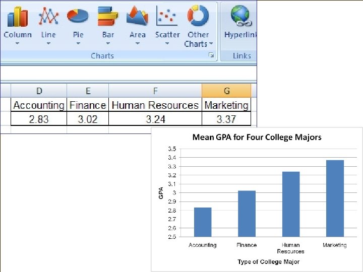
Type of major in school 4 (accounting, finance, hr, marketin Homework Grade Point Average 0. 05 2. 83 3. 02 3. 24 3. 37

If observed F is bigger than critical F: F: If observed F is bigger critical Reject null & Significant! Homework If p value is less than 0. 05: Reject null & Significant! 4 -1=3 # groups - 1 # scores - number of groups 28 - 4=24 # scores - 1 28 - 1=27 0. 3937 0. 1119 0. 3937 / 0. 1119 = 3. 517 3. 009 3 24 0. 03

Yes Homework F (3, 24) = 3. 517; p < 0. 05 The GPA for four majors was compared. The average GPA was 2. 83 for accounting, 3. 02 for finance, 3. 24 for HR, and 3. 37 for marketing. An ANOVA was conducted and there is a significant difference in GPA for these four groups (F(3, 24) = 3. 52; p < 0. 05).

Number of observations in each group Average for each group (We REALLY care about this one)

“SS” = “Sum of Squares” - will be given for exams Number of groups minus one (k – 1) 4 -1=3 Number of people minus number of groups (n – k) 28 -4=24

SS between df between SS within df within MS between MS within

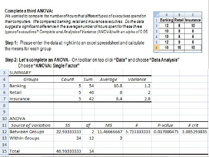
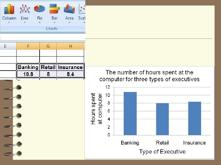
Type of executive 3 (banking, retail, insurance) Hours spent at computer 0. 05 10. 8 8 8. 4

If observed F is bigger than critical F: F: If observed F is bigger than critical Reject null & Significant! If p value is less than 0. 05: Reject null & Significant! 11. 46 2 11. 46 / 2 = 5. 733 3. 88 2 12 0. 0179

Yes F (2, 12) = 5. 73; p < 0. 05 The number of hours spent at the computer was compared for three types of executives. The average hours spent was 10. 8 for banking executives, 8 for retail executives, and 8. 4 for insurance executives. An ANOVA was conducted and we found a significant difference in the average number of hours spent at the computer for these three groups , (F(2, 12) = 5. 73; p < 0. 05).

Number of observations in each group Average for each group Just add up all scores

“SS” = “Sum of Squares” - will be given for exams Number of groups minus one (k – 1) 3 -1=2 Number of people minus number of groups (n – k) 15 -3=12

SS between df between SS within df within MS between MS within