Introduction to Statistics for the Social Sciences SBS

Introduction to Statistics for the Social Sciences SBS 200, COMM 200, GEOG 200, PA 200, POL 200, or SOC 200 Lecture Section 001, Spring 2015 Room 150 Harvill Building 8: 00 - 8: 50 Mondays, Wednesdays & Fridays.

Labs continue this week with Multiple Regression

Schedule of readings Before next exam (Monday May 4 th) Please read chapters 10 – 14 Please read Chapters 17, and 18 in Plous Chapter 17: Social Influences Chapter 18: Group Judgments and Decisions

Homework due – Monday (April 27 th) On class website: Homeworksheet #20 Creating multiple choice questions Please note: - No class on Friday – - A morning of rest Extra Credit Opportunity

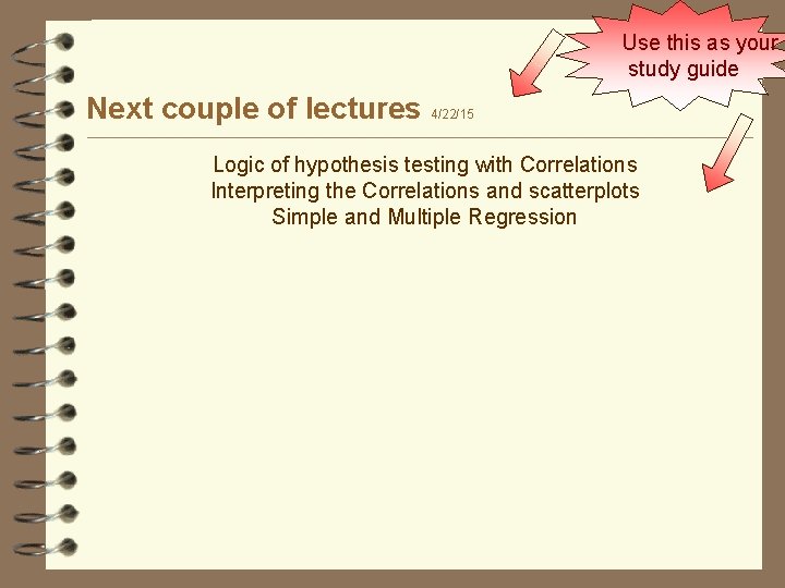
Use this as your study guide Next couple of lectures 4/22/15 Logic of hypothesis testing with Correlations Interpreting the Correlations and scatterplots Simple and Multiple Regression

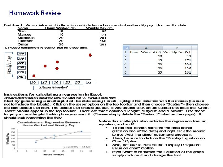
Homework Review

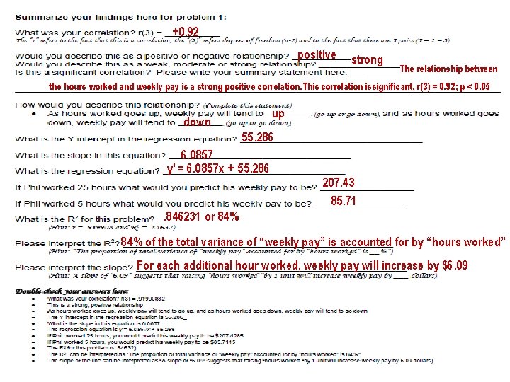
+0. 92 positive strong The relationship between the hours worked and weekly pay is a strong positive correlation. This correlation issignificant, r(3) = 0. 92; p < 0. 05 up down 55. 286 6. 0857 y' = 6. 0857 x + 55. 286 207. 43 85. 71 . 846231 or 84% of the total variance of “weekly pay” is accounted for by “hours worked” For each additional hour worked, weekly pay will increase by $6. 09

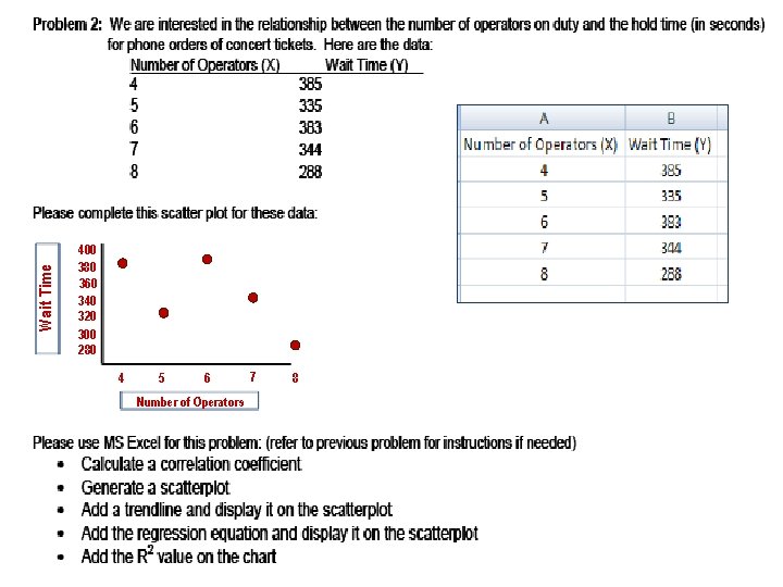
Wait Time 400 380 360 340 320 300 280 4 5 6 Number of Operators 7 8

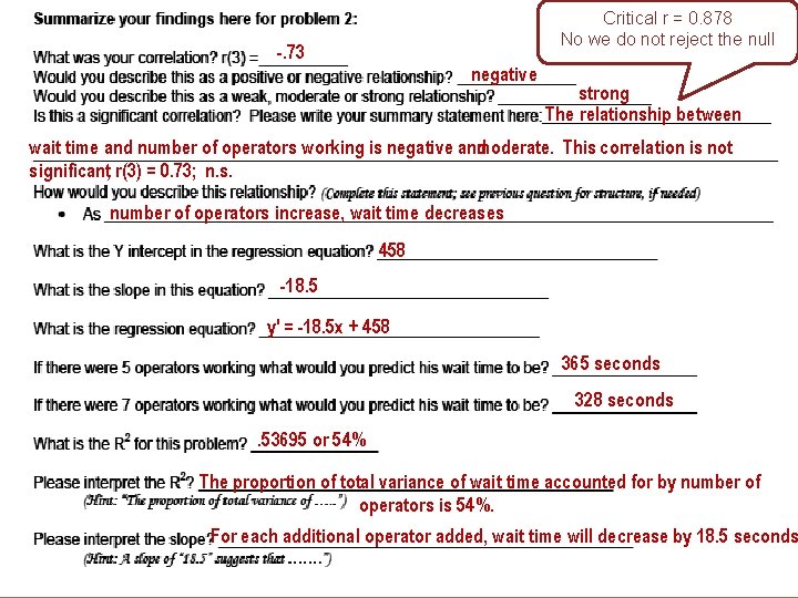
Critical r = 0. 878 No we do not reject the null -. 73 negative strong The relationship between wait time and number of operators working is negative and moderate. This correlation is not significant, r(3) = 0. 73; n. s. number of operators increase, wait time decreases 458 -18. 5 y' = -18. 5 x + 458 365 seconds 328 seconds. 53695 or 54% The proportion of total variance of wait time accounted for by number of operators is 54%. For each additional operator added, wait time will decrease by 18. 5 seconds

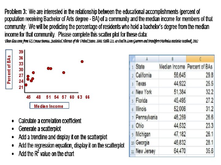
Percent of BAs 39 36 33 30 27 24 21 45 48 51 54 57 60 63 66 Median Income

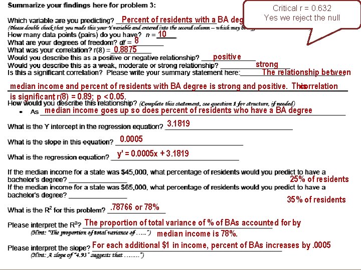
Percent of residents with a BA degree 8 0. 8875 Critical r = 0. 632 Yes we reject the null 10 positive strong The relationship between median income and percent of residents with BA degree is strong and positive. This correlation is significant, r(8) = 0. 89; p < 0. 05. median income goes up so does percent of residents who have a BA degree 3. 1819 0. 0005 y' = 0. 0005 x + 3. 1819 25% of residents. 78766 or 78% 35% of residents The proportion of total variance of % of BAs accounted for by median income is 78%. For each additional $1 in income, percent of BAs increases by. 0005

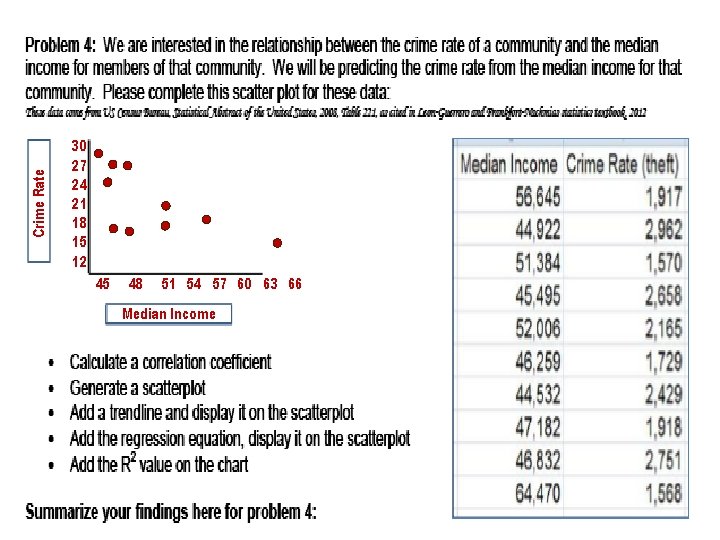
Crime Rate 30 27 24 21 18 15 12 45 48 51 54 57 60 63 66 Median Income

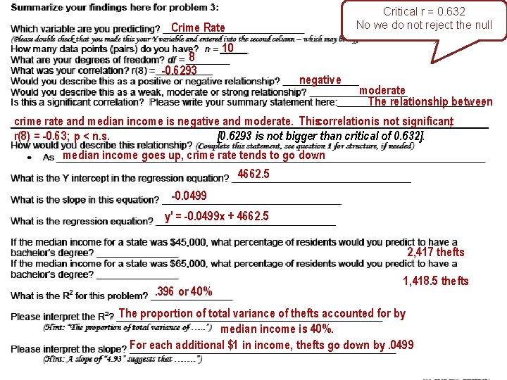
Critical r = 0. 632 No we do not reject the null Crime Rate 8 -0. 6293 10 negative moderate The relationship between crime rate and median income is negative and moderate. Thiscorrelation is not significant, r(8) = -0. 63; p < n. s. [0. 6293 is not bigger than critical of 0. 632]. median income goes up, crime rate tends to go down 4662. 5 -0. 0499 y' = -0. 0499 x + 4662. 5 2, 417 thefts. 396 or 40% 1, 418. 5 thefts The proportion of total variance of thefts accounted for by median income is 40%. For each additional $1 in income, thefts go down by. 0499

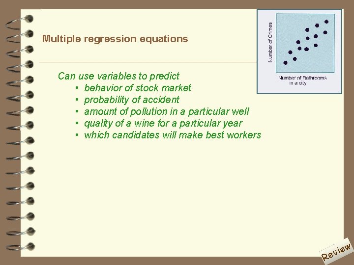
Multiple regression equations Can use variables to predict • behavior of stock market • probability of accident • amount of pollution in a particular well • quality of a wine for a particular year • which candidates will make best workers R w e evi

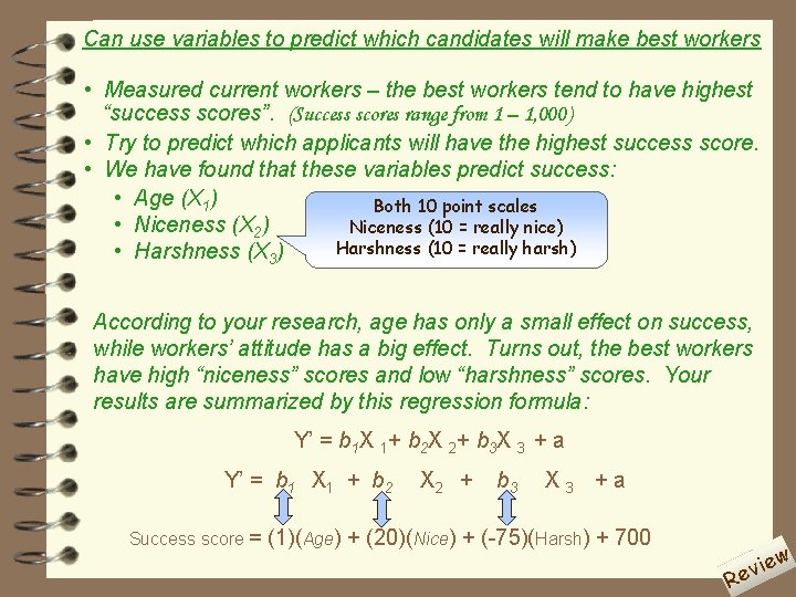
Can use variables to predict which candidates will make best workers • Measured current workers – the best workers tend to have highest “success scores”. (Success scores range from 1 – 1, 000) • Try to predict which applicants will have the highest success score. • We have found that these variables predict success: • Age (X 1) Both 10 point scales • Niceness (X 2) Niceness (10 = really nice) Harshness (10 = really harsh) • Harshness (X 3) According to your research, age has only a small effect on success, while workers’ attitude has a big effect. Turns out, the best workers have high “niceness” scores and low “harshness” scores. Your results are summarized by this regression formula: Y’ = b 1 X 1+ b 2 X 2+ b 3 X 3 + a Y’ = b 1 X 1 + b 2 Success score = X 2 + b 3 X 3 +a (1)(Age) + (20)(Nice) + (-75)(Harsh) + 700 R w e evi

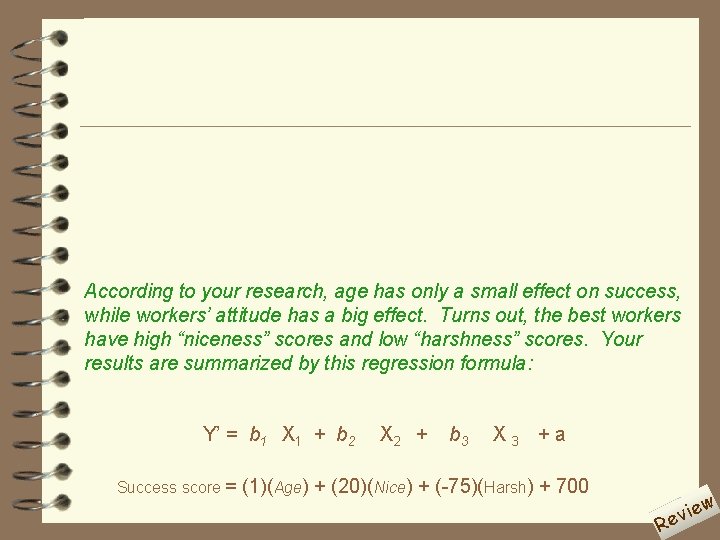
According to your research, age has only a small effect on success, while workers’ attitude has a big effect. Turns out, the best workers have high “niceness” scores and low “harshness” scores. Your results are summarized by this regression formula: Y’ = b 1 X 1 + b 2 Success score = X 2 + b 3 X 3 +a (1)(Age) + (20)(Nice) + (-75)(Harsh) + 700 R w e evi

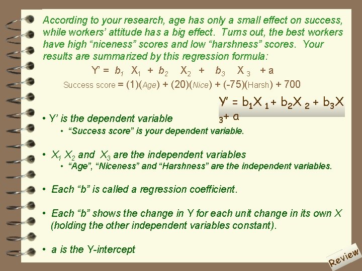
According to your research, age has only a small effect on success, while workers’ attitude has a big effect. Turns out, the best workers have high “niceness” scores and low “harshness” scores. Your results are summarized by this regression formula: Y’ = b 1 X 1 + b 2 X 2 + b 3 X 3 + a Success score = (1)(Age) + (20)(Nice) + (-75)(Harsh) + 700 • Y’ is the dependent variable Y’ = b 1 X 1 + b 2 X 2 + b 3 X 3+ a • “Success score” is your dependent variable. • X 1 X 2 and X 3 are the independent variables • “Age”, “Niceness” and “Harshness” are the independent variables. • Each “b” is called a regression coefficient. • Each “b” shows the change in Y for each unit change in its own X (holding the other independent variables constant). • a is the Y-intercept R w e evi

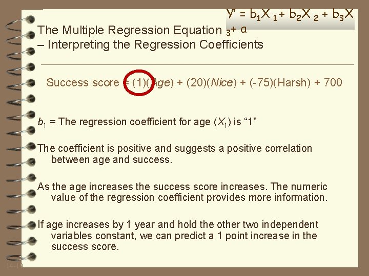
Y’ = b 1 X 1 + b 2 X 2 + b 3 X The Multiple Regression Equation 3+ a – Interpreting the Regression Coefficients Success score = (1)(Age) + (20)(Nice) + (-75)(Harsh) + 700 b 1 = The regression coefficient for age (X 1) is “ 1” The coefficient is positive and suggests a positive correlation between age and success. As the age increases the success score increases. The numeric value of the regression coefficient provides more information. If age increases by 1 year and hold the other two independent variables constant, we can predict a 1 point increase in the success score. 14 -19

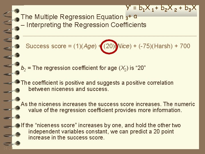
Y’ = b 1 X 1 + b 2 X 2 + b 3 X The Multiple Regression Equation 3+ a – Interpreting the Regression Coefficients Success score = (1)(Age) + (20)(Nice) + (-75)(Harsh) + 700 b 2 = The regression coefficient for age (X 2) is “ 20” The coefficient is positive and suggests a positive correlation between niceness and success. As the niceness increases the success score increases. The numeric value of the regression coefficient provides more information. If the “niceness score” increases by one, and hold the other two independent variables constant, we can predict a 20 point increase in the success score. 14 -20

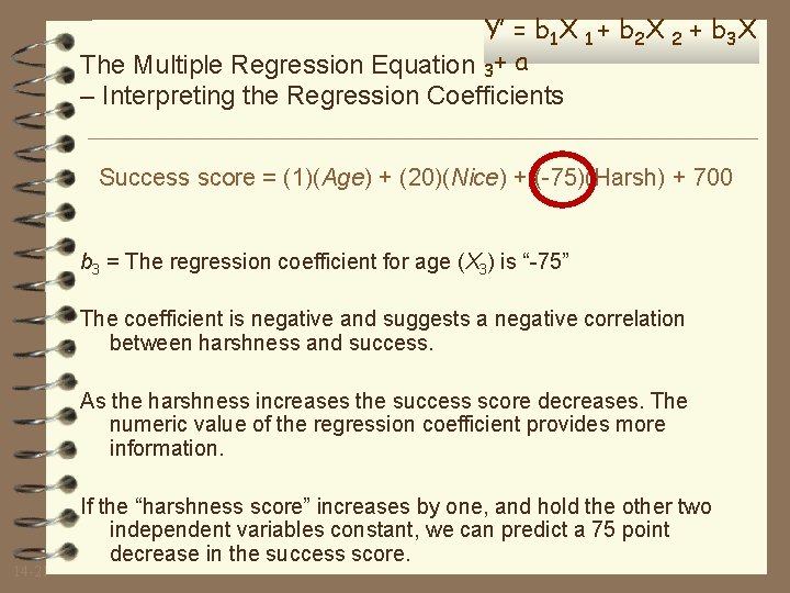
Y’ = b 1 X 1 + b 2 X 2 + b 3 X The Multiple Regression Equation 3+ a – Interpreting the Regression Coefficients Success score = (1)(Age) + (20)(Nice) + (-75)(Harsh) + 700 b 3 = The regression coefficient for age (X 3) is “-75” The coefficient is negative and suggests a negative correlation between harshness and success. As the harshness increases the success score decreases. The numeric value of the regression coefficient provides more information. 14 -21 If the “harshness score” increases by one, and hold the other two independent variables constant, we can predict a 75 point decrease in the success score.

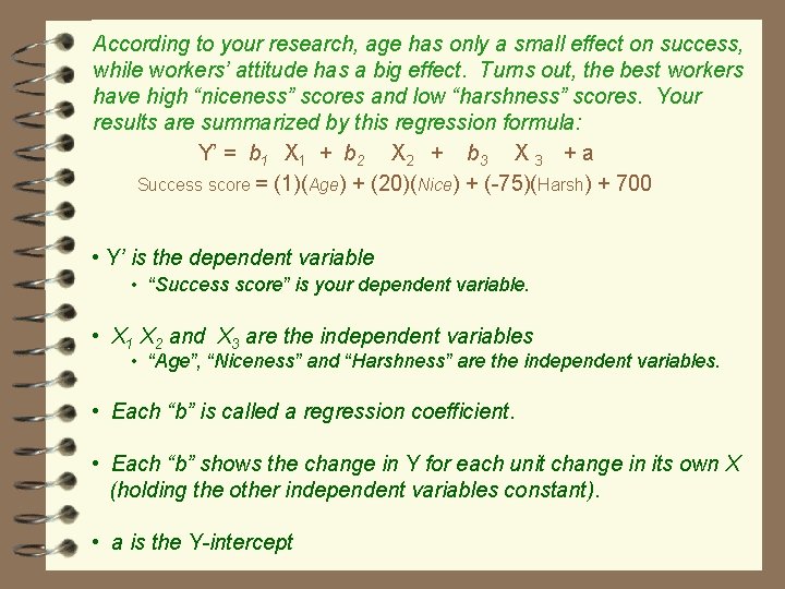
According to your research, age has only a small effect on success, while workers’ attitude has a big effect. Turns out, the best workers have high “niceness” scores and low “harshness” scores. Your results are summarized by this regression formula: Y’ = b 1 X 1 + b 2 X 2 + b 3 X 3 + a Success score = (1)(Age) + (20)(Nice) + (-75)(Harsh) + 700 • Y’ is the dependent variable • “Success score” is your dependent variable. • X 1 X 2 and X 3 are the independent variables • “Age”, “Niceness” and “Harshness” are the independent variables. • Each “b” is called a regression coefficient. • Each “b” shows the change in Y for each unit change in its own X (holding the other independent variables constant). • a is the Y-intercept

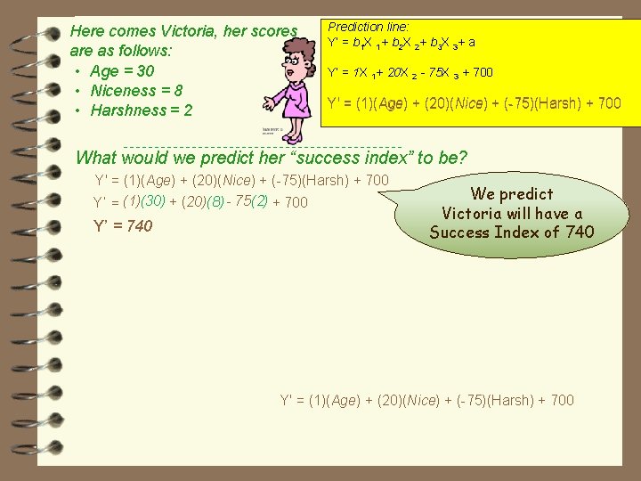
Here comes Victoria, her scores are as follows: • Age = 30 • Niceness = 8 • Harshness = 2 Prediction line: Y’ = b 1 X 1+ b 2 X 2+ b 3 X 3+ a Y’ = 1 X 1+ 20 X 2 - 75 X 3 + 700 Y' = (1)(Age) + (20)(Nice) + (-75)(Harsh) + 700 What would we predict her “success index” to be? Y' = (1)(Age) + (20)(Nice) + (-75)(Harsh) + 700 Y’ = (1)(30) + (20)(8) - 75(2) + 700 Y’ = 740 We predict Victoria will have a = 3. 812 Success Index of 740 Y' = (1)(Age) + (20)(Nice) + (-75)(Harsh) + 700

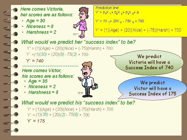
Here comes Victoria, her scores are as follows: • Age = 30 • Niceness = 8 • Harshness = 2 Prediction line: Y’ = b 1 X 1+ b 2 X 2+ b 3 X 3+ a Y’ = 1 X 1+ 20 X 2 - 75 X 3 + 700 Y' = (1)(Age) + (20)(Nice) + (-75)(Harsh) + 700 What would we predict her “success index” to be? Y' = (1)(Age) + (20)(Nice) + (-75)(Harsh) + 700 Y’ = (1)(30) + (20)(8) - 75(2) + 700 Y’ = 740 = 3. 812 Here comes Victor, his scores are as follows: • Age = 35 • Niceness = 2 • Harshness = 8 We predict Victoria will have a Success Index of 740 We predict Victor will have a Success Index of 175 What would we predict his “success index” to be? Y' = (1)(Age) + (20)(Nice) + (-75)(Harsh) + 700 Y’ = (1)(35) + (20)(2) - 75(8) + 700 Y’ = 175

Can use variables to predict which candidates will make best workers We predict Victor will have a Success Index of 175 We predict Victoria will have a Success Index of 740 Who will we hire?