Introduction to statistics and SPSS A little about

Introduction to statistics and SPSS

A little about me, Dr. Natalie Wright �Undergraduate degree in psychology from Colorado State University �Ph. D. in industrial and organizational psychology from North Carolina State University

My research �My research focuses on several different areas: �Evaluation of psychological measurements in organizational contexts �Work analysis and the changing nature of work across time and culture �Humanitarian work psychology

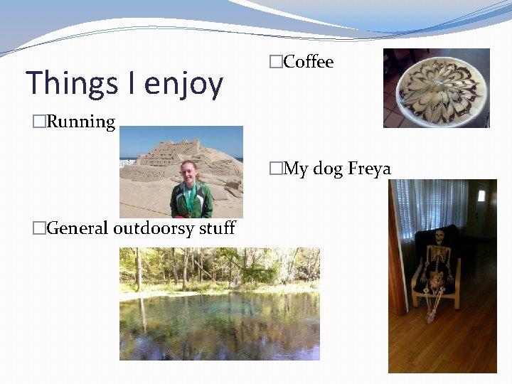
Things I enjoy �Coffee �Running �My dog Freya �General outdoorsy stuff

Learning about you �What is your name? �What year are you in the program? �What is your undergraduate degree? Where did you graduate? �Where are you from? �What are your primary interests in your field? �What are you hoping to get out of this class?

The syllabus

Basic research and statistics review

Research approaches �Experimental: involves manipulating independent variable and measuring its effect on the dependent variable �Randomized experimental: participants randomly assigned to conditions �Quasi-experimental: participants not randomly assigned to conditions

Research approaches �Nonexperimental research: no manipulation of independent variable �Comparative approach: compare groups on some naturally-occurring variable (gender, age, etc. ) �Associational approach: measure several variables and evaluate relationships between them (correlational)

Variables �Variable: something that can be measured �Examples: personality, gender, reaction time, intelligence �A variable has to vary � If all participants in study were female, then gender wasn’t a variable

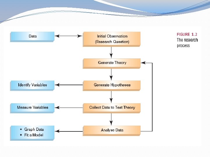
Theories & hypotheses �Theory: explanation of phenomenon (broad generalizations) �Should produce testable hypotheses �Example: Students who study hard will do well in class. �Hypothesis: testable statement derived from theory (actual prediction of outcome) �Must be testable �Prediction of what will happen �Example: Students who study for 10 or more hours per week will have significantly higher test scores than students who study for 5 hours or less per week

Theories & hypotheses �All theories and hypotheses must be falsifiable: able to be proved wrong �Clearly defined variables in theories and hypotheses �Falsifiable theory: Religious individuals have lower stress than non-religious individuals �Non-falsifiable theory: Religious individuals lead better lives than non-religious individuals

Independent variable �Proposed causal variable �Variable that is manipulated in experiment �Example: Training type: online vs. classroom �Or, in correlational study: predictor variable �Training self-efficacy

Dependent variable �Proposed outcome/effect variable �What changes in response to independent variable �In experimental study, variable that is expected to change due to experimental manipulation �Example: training performance �In correlational study, outcome variable �Example: training performance

Levels of measurement �Categorical variables: have distinct categories �Nominal variable: purely categorical: no numerical value � Example: Gender � Confusing example: wrong/right items: categorical, but ability underlying responses is continuous � Underlying trait is continuous when using correct/incorrect (Ex: Knowledge of research design) �Ordinal variable: Rank ordered, but distance between ranks not always equal � Example: runners in a half marathon: winner ran a 1: 12: 03, 2 nd place ran a 1: 12: 05, 3 rd place ran a 1: 17: 18

Levels of measurement �Continuous variables �Interval variable: equal intervals between each value, but no true zero � Has arbitrary zero-doesn’t show total lack of trait � Example: intelligence measured with WAIS: zero doesn’t mean absolutely no intelligence �Ratio variable: equal intervals between each value, has true zero � Zero means total lack of whatever is being measured � Example: Kelvin scale of temperature � No psychological measurement has ratio-level measurement

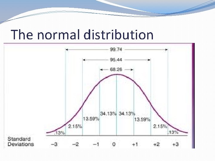
The normal distribution

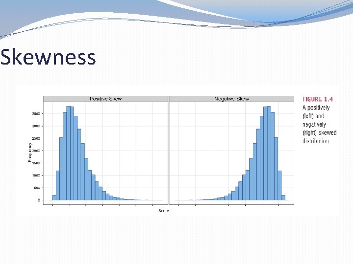
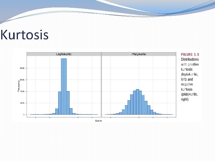
Frequency distributions �Skew �Symmetry of distribution �Kurtosis �Peakiness of distribution � Flat vs pointy

Skewness

Kurtosis

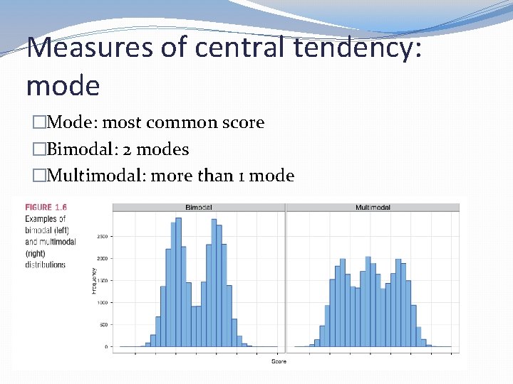
Measures of central tendency: mode �Mode: most common score �Bimodal: 2 modes �Multimodal: more than 1 mode

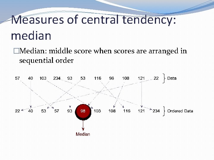
Measures of central tendency: median �Median: middle score when scores are arranged in sequential order

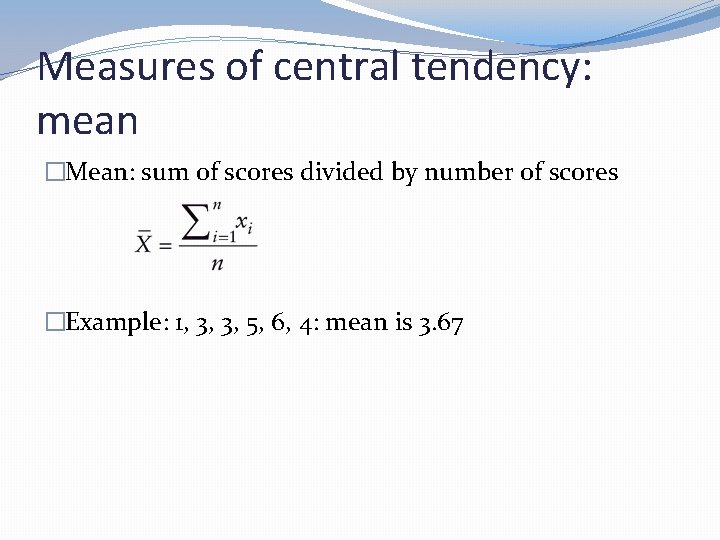
Measures of central tendency: mean �Mean: sum of scores divided by number of scores �Example: 1, 3, 3, 5, 6, 4: mean is 3. 67

Measures of variability: range �Range: highest score – lowest score � 1, 3, 5, 9, 10: range is 9

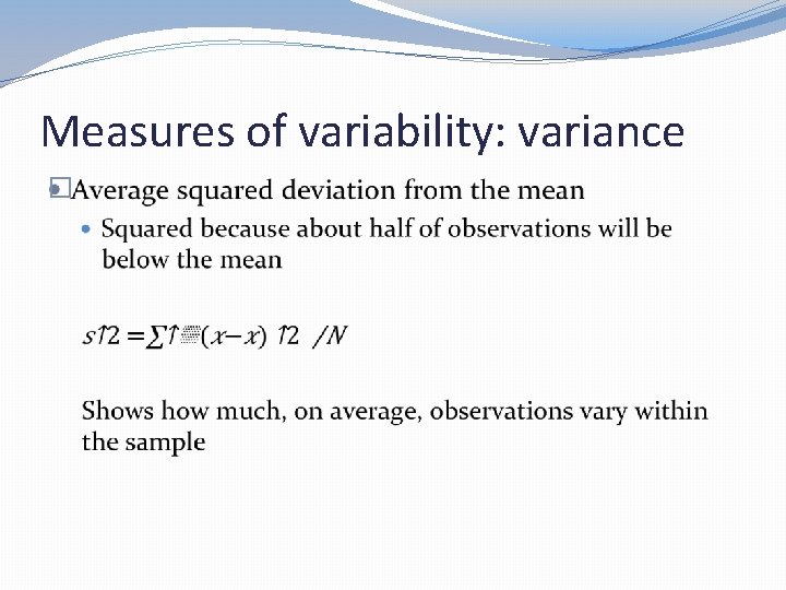
Measures of variability: variance �

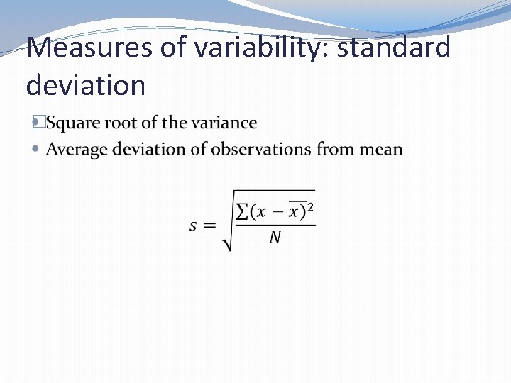
Measures of variability: standard deviation �

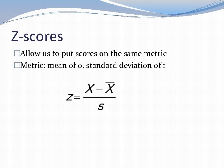
Z-scores �Allow us to put scores on the same metric �Metric: mean of 0, standard deviation of 1

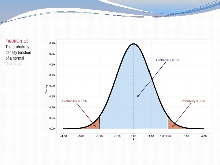
Properties of z-scores � 1. 96 cuts off the top 2. 5% of the distribution. �− 1. 96 cuts off the bottom 2. 5% of the distribution. �As such, 95% of z-scores lie between − 1. 96 and 1. 96. � 99% of z-scores lie between − 2. 58 and 2. 58, � 99. 9% of them lie between − 3. 29 and 3. 29.

Statistical models

Statistical model �Want to learn about real-world phenomenon �Collect data to test hypotheses about phenomenon �Testing hypotheses requires building statistical models �Do students who study 10 hours per week have a higher GPA than students who study 5 hours per week? � Compare means �Is training self-efficacy related to training performance? � Regression model

Statistical model �Fit: degree to which statistical model represents data collected (just hypothesis testing) �Good fit: hypothesized model closely fits real world � Students who study 10 hours per week do indeed have higher GPAs than those who study 5 hours per week �Bad fit: hypothesized model doesn’t resemble what happens in real world � Students who study 10 hours per week have lower those who study 5 hours per week GPAs than

Population vs. sample �Population: entire group to which we want to generalize our findings �All college students �All working-age adults in job retraining programs, etc. �Sample: group that we actually collect data from � 200 students at Valdosta State University � 300 adults in job retraining programs in Lowndes County

Population vs. sample �Ideally, want to generalize findings from sample to population �To do this, sample needs to approximate population �Bigger samples tend to be better for this �Beware of ways in which sample may vary markedly from population � What if students at Valdosta State are more intelligent than college students in rest of US?

General equation for statistical models �ALL statistical models boil down to this:

Parts of model �Variables: things that we measure �Parameters: estimated from the data: represent relationships between variables in the population �Use sample to estimate population parameters

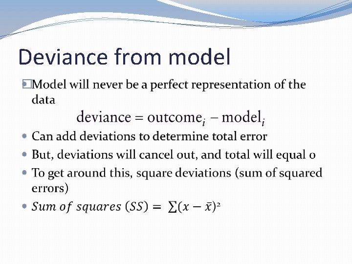
Deviance from model �

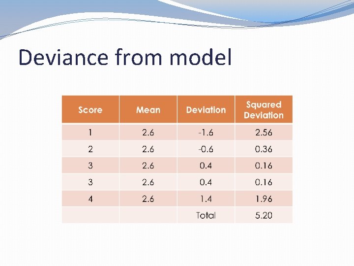
Deviance from model

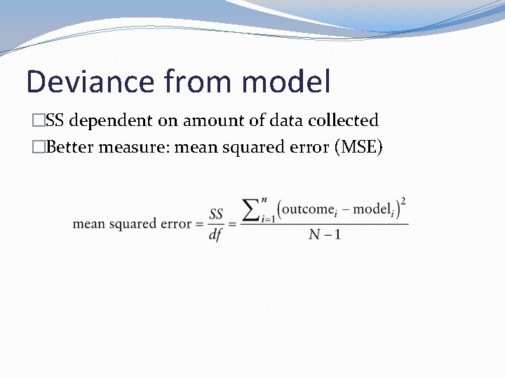
Deviance from model �SS dependent on amount of data collected �Better measure: mean squared error (MSE)

Degrees of freedom �Abbreviated df �Degrees of freedom: number of observations that are free to vary without changing value �If we hold a parameter constant (such as mean when calculating MSE), not all scores used to calculate that parameter are free to vary without changing parameter value �Example: calculated mean from 5 scores: 2, 3, 4, 8, 8: mean=5 � 4 of these scores can vary, but 1 needs to be held constant to ensure mean stays same �Thus, df=4

Sampling distribution �Sampling variation: if we took several different samples from population, each would vary �Different members of population �Could (hypothetically) draw infinite number of samples from population and estimate parameter of interest for each sample �Frequency distribution of these parameter values: sampling distribution �Mean of distribution: value of parameter for population �Sampling distributions hypothetical

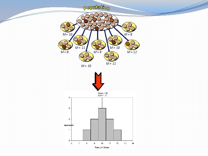
= 10 M=9 M = 11 M=9 M = 10 M=8 M = 10 M = 12 M = 11

Standard error �Standard deviation: shows how far away from the mean each observation in a sample is �Standard error: like standard deviation for samples �Standard error: how far away from mean of sampling distribution the parameter estimate for a sample is �Large standard error: estimated parameter not very good estimate of population parameter � Sample is different from population �Small standard error: estimated parameter good estimate of population parameter � Sample more closely represents population

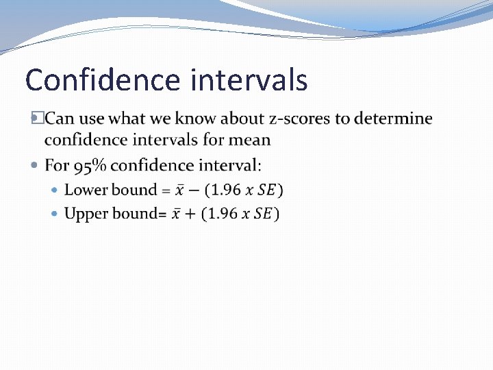
Confidence intervals �Boundary in which we are X% confident that population parameter falls �Usually create 95% confidence intervals �Need to determine limits which X% of parameter values will fall in sampling distribution �From central limit theorem: in samples of at least 30, sampling distribution will be normally distributed

Confidence intervals �

Types of hypotheses �Null hypothesis (H 0) �There is no effect �Example: Training self-efficacy doesn’t predict training performance �Alternative (research) hypothesis (H 1) �There is an effect �Example: Training self-efficacy does predict training performance

Null hypothesis significance testing (NHST) �Assume that null hypothesis is true �Fit statistical model to data that represents alternative hypothesis and see how well it fits �Calculate probability of getting test statistic if null hypothesis was true �If probability small (convention: <. 05, or 5%), assume it’s unlikely that the null hypothesis was true �Find support for alternative hypothesis �But you never “prove” alternative hypothesis

Test statistics �Test statistic: statistic for which frequency of values is known �Examples: t, F, χ2 �Distribution for statistic is known �Observed values can be used to test hypothesis �Test statistic is ratio of systematic variation (explained by model) and unsystematic variation (not explained by model)

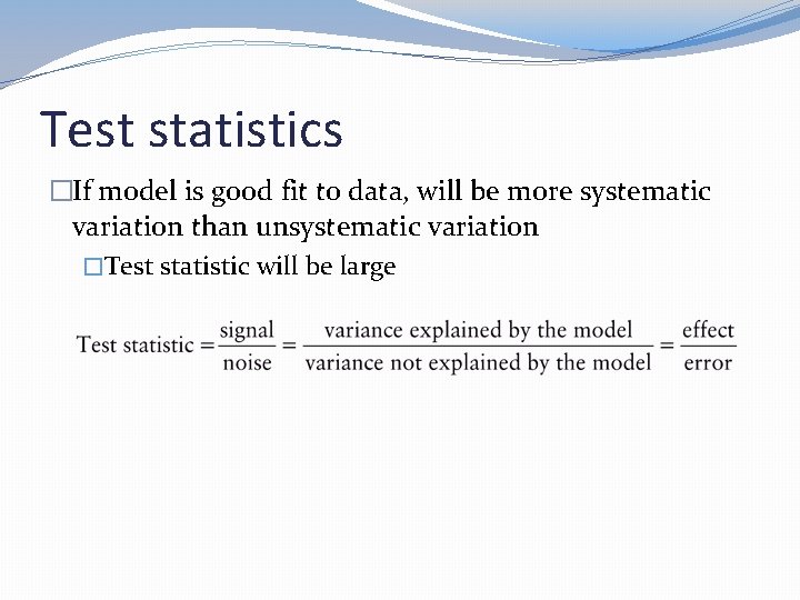
Test statistics �If model is good fit to data, will be more systematic variation than unsystematic variation �Test statistic will be large

Null hypothesis significance testing (NHST)

One and two tailed tests �Hypotheses can be directional or non-directional �Non-directional: students who study for 10 hours per week will have a different GPA than students who study for 5 hours per week �Directional: students who study for 10 hours per week will have a higher GPA than students who study for 5 hours per week

One and two tailed tests �Directionality of hypothesis relates to critical value for test statistic �One-tailed: lower critical value to reject null hypothesis (directional) �But, if you were wrong on direction, you’ll have a nonsignificant finding �Two-tailed: higher critical value to reject null hypothesis (non-directional) �But, doesn’t matter which way effect occurs: can hedge your bets �No cheating! Pick directionality before doing analyses

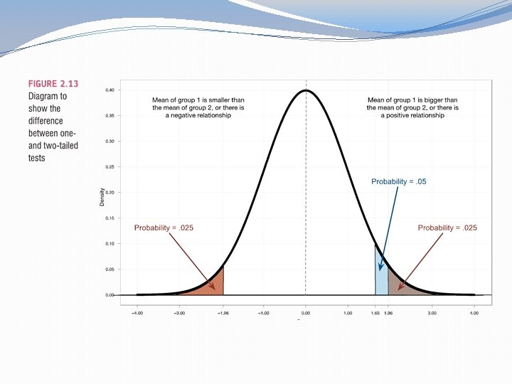
One and two tailed tests �Decision should be based on theory/previous literature �If theory/previous research doesn’t show strong support either way: two tailed �If theory/previous literature strongly suggests clear, directional difference: one tailed

Type I and Type II errors �Type I error: saying there is an effect when there isn’t �Determined by our p-value (set before analyses; 0. 05)/α level �If we stick to. 05 cutoff, then probability of Type I error is 5% �Type II error: saying that there isn’t an effect when there is �Determined by β (which is related to power-we’ll get there in a minute) �Ideal level: . 20 (or 20%)

Statistical power �Power of test: probability that test will find an effect that truly exists in population �Power = 1 -β �Ideal power: . 80 or above �Power depends on: �Size of effect: big effects easier to find �α level: lower alpha = less power �Sample size: larger samples = more power

Problems with NHST �Promotes dichotomous thinking: significant vs. not significant �Publication bias � Bias meta-analytic results � Focus on works that are published �p value tells probability of finding results we did if null hypothesis true �Tend to interpret this as probability that null hypothesis is true, which isn’t same �At high levels of power, almost anything significant �Statistical significance vs. practical significance

Sample size and NHST �As sample size goes up, it’s easier and easier to reject null hypothesis �To a point, this is good �But with extremely large sample size: tiny, trivial differences will be statistically significant �Tiny difference between means may not be practically significant

Effect sizes �Effect size: standardized measure of effect �Can be compared across studies �Not as influenced by sample size as test statistics and their associated p-values �Better measure of the actual importance of an effect �More on effect sizes later

Statistical bias

3 kinds of bias we worry about �Things that bias parameter estimates �Things that bias standard errors and confidence intervals �Things that bias test statistics and p-values �These aren’t isolated �Example: Test statistic values may be affected by standard error

Sources of bias �Bias generally happens due to: �Violation of assumptions of statistical tests �Outliers

Assumptions �Statistical tests make assumptions about the data �If these are violated, test statistic and p-value will not be accurate �Tests have own assumptions �Most linear models have similar assumptions

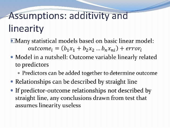
Assumptions �Parametric statistical tests based on normal distribution �Most of tests that we use (t-test, ANOVA, regression, etc. ) are parametric �Assumptions �Additivity and linearity �Normality of some aspect of data �Homoscedasticity/homogeneity of variance �Independence of observations

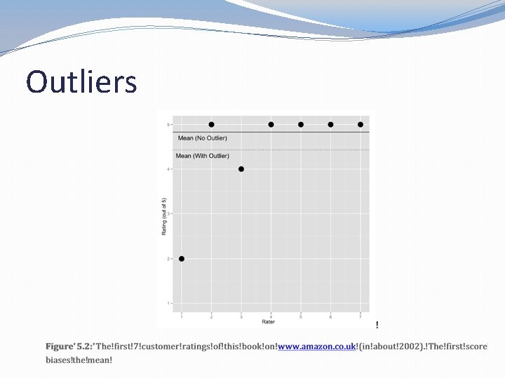
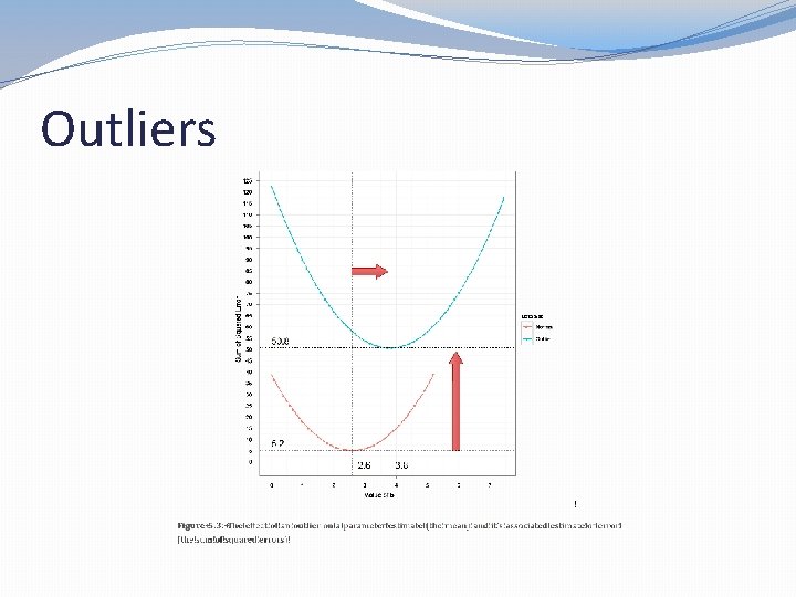
Outliers �Outlier: score very different than rest of data �Example: 4, 5, 6, 3, 4, 5, 3, 4, 17 �Strange scores can bias parameter estimates �Using scores from above: mean = 5. 67 �Without score of 17, mean = 4. 25 �Sum of squared error is affected even more: �With outlier: SS = 152. 001 �Without outlier: SS = 7. 5

Outliers

Outliers

Assumptions: additivity and linearity �

Nonlinear relationship

Assumptions: normality �Normal distribution related to: �Parameter estimates � Skewed distributions influence parameter estimates �Confidence intervals � Calculated using standard error, which relates to normal distribution �Null hypothesis significance testing � Assume parameter estimates have normal distribution �Errors � Deviance from model-estimated values should be normally distributed

Assumptions: normality �Does not mean your data has to be normally distributed �Confidence intervals around parameter estimate assume normal distribution, but: �Model significance tests assume sampling distribution for value being tested is normal �Good parameter estimates rely on errors that are normally distributed

Assumptions: normality �From central limit theorem: sampling distribution of parameter estimate approaches normality when sample = 30 or higher (usually) �So, usually if sample large enough, don’t need to worry about normality �Fitting model using method of least squares (what we usually do) tends to result in normally distributed error

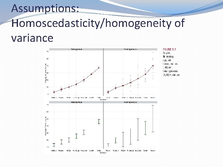
Assumptions: Homoscedasticity/homogeneity of variance �Homogeneity of variance/homoscedasticity of variance: variance (spread) of scores for the outcome variable equal at all levels of the predictor �If comparing groups (t-tests, ANOVAs), samples should come from populations with equal variance

Assumptions: Homoscedasticity/homogeneity of variance

Assumptions: Homoscedasticity/homogeneity of variance �Method of least squares (for estimating parameters) gives best estimates if variance of outcome variable equivalent across all levels of predictor(s) �NHST gives accurate test statistics only if variance of outcome equal across levels of predictor

Assumptions: independence �Errors in model not correlated with one another �If responses aren’t independent (participants talked to each other before giving answers, participant took survey twice, etc. ) then errors will be correlated �If errors aren’t independent: �Inaccurate confidence intervals � Rely on calculating standard error � Ensure observations are independent of each other to decrease inaccuracy �Inaccurate statistical tests

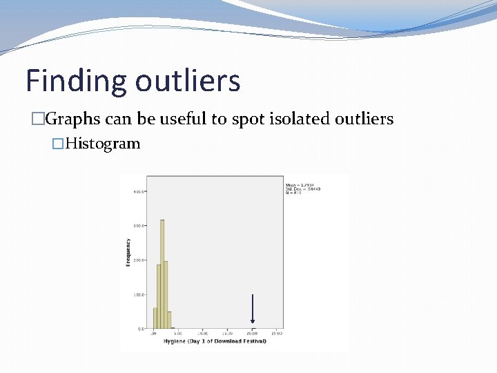
Finding outliers �Graphs can be useful to spot isolated outliers �Histogram

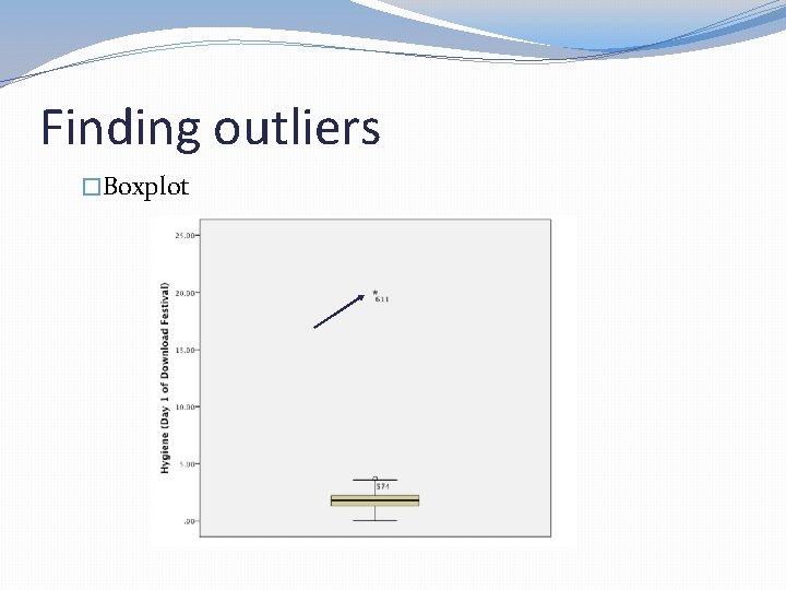
Finding outliers �Boxplot

Finding outliers �If you have one isolated outlier �Double-check your data! �Likely coding/data entry mistake

Finding outliers �Transforming scores to z-scores allows you to check for outliers �Steps: �In descriptives tab, choose variables of interest and then check “Save standardized values as variables” box �Determine cutoff for what you consider an “outlier. ” Options include: � > absolute value of 3. 29: 99. 9% of scores will fall below this � >3 SD away from mean

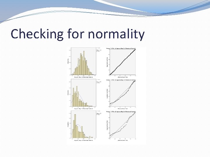
Checking for normality �P-P (probability-probability) plot: plots cumulative probability of variable against cumulative probability of distribution �Data normally distributed: straight line �Not normally distributed: data falls below or above straight line

Checking for normality

Checking for normality �Go to “descriptive statistics, ” and choose “frequencies” �From there: �Click on “statistics” �Choose “kurtosis” and “skewness”

Checking for normality �Skewness: �Positive values: Lots of scores at lower end of distribution �Negative values: Lots of scores at higher end of distribution �Kurtosis: �Positive values: Pointy distribution �Negative values: Flat distribution �Larger values (further from 0): data not normally distributed

Checking for normality �Kolgorov-Smirnov test & Shapiro-Wilk test �Compare scores in sample to normally distributed set of scores with same mean and SD �Test non-significant: scores not significantly different from normal distribution �Test significant: scores significantly different from normal distribution �Access these tests from “descriptive statistics” – “explore”

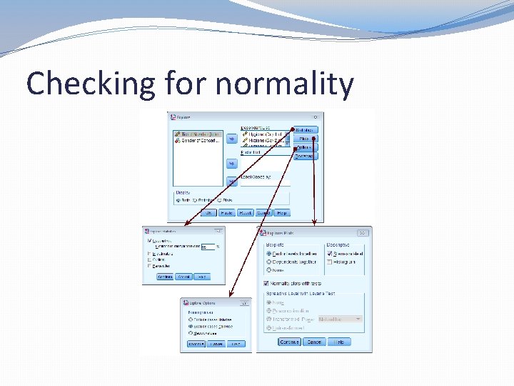
Checking for normality

Checking for normality �If comparing means for multiple groups, need to check normality within each group �To do this, go to “data, ” then “split file” �Pull relevant grouping variable into box �Check “organize output by groups” �Analyses will now be run separately for each group �Make sure to turn this option off before you make the mean comparisons!

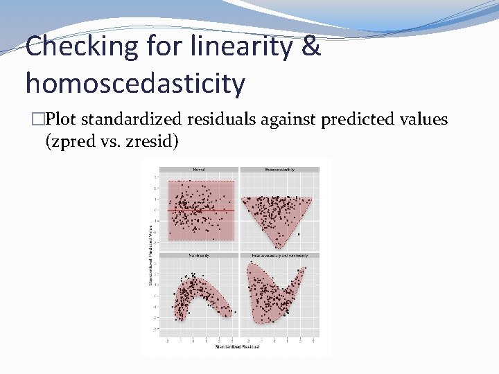
Checking for linearity & homoscedasticity �Plot standardized residuals against predicted values (zpred vs. zresid)

Checking for homoscedasticity �Levene’s test: does one-way ANOVA on deviance scores across groups �If significant, homogeneity of variance assumption violated �Accessed through “descriptive statistics” – “explore” – “plots” �Unless data transformed, choose “untransformed”

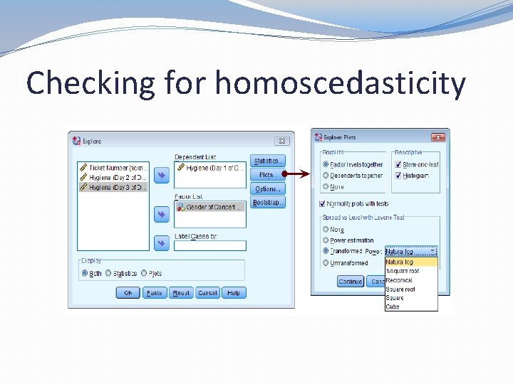
Checking for homoscedasticity

Ways to reduce bias �Trim data �Delete certain amount of extreme scores �Winsorize data �Substitute outliers with highest value that isn’t outlier �Analyze data with robust methods �Bootstrapping �Transform data �Apply mathematical function to scores to correct problems

Ways to reduce bias �Trimming data �Don’t automatically remove outliers: only do so if there’s reason to think they come from different population � 2 general rules for data trimming: �Percentage based (example: remove 5% of highest and lowest scores) �Standard deviation based (example: remove all scores more than 3 sds away from mean) � Problem: extreme scores were used to calculate sd

Ways to reduce bias �Winsorizing �Replace outlier with next highest score that isn’t an outlier �Robust methods �Involves using tests that aren’t greatly affected by non- normal data �Non-parametric methods: don’t have assumption of normally distributed data �Bootstrapping: sample data treated as population Smaller samples drawn repeatedly from population � Calculates parameter estimates for each bootstrap sample � Confidence intervals calculated for bootstrap samples �

Ways to reduce bias �Transforming data: use equation to change every score to get rid of distributional problems �Changes the form of relationships between variables �Relative differences between participants don’t change �For correlations: just change problematic variable �For differences between variables: change all variables �Problems with transformation: �Changes the hypothesis that you’re testing �Using wrong transformation worse than no transformation at all

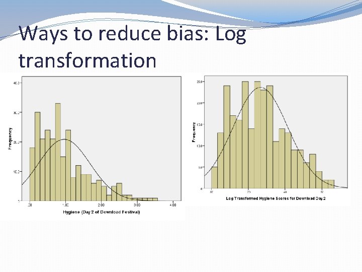
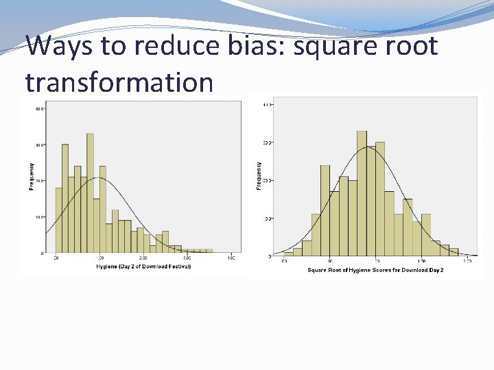
Ways to reduce bias �Log transformation: take logarithm of scores �Flattens positive tail of distribution �Doesn’t work for 0 or negative numbers �Helps correct for positive skew, positive kurtosis, unequal variances, non-linear data �Square root transformation: take square root of scores �Brings smaller scores closer to the center: larger effect of big scores than small scores �Only works to fix positive outliers-can’t take square root of negative number �Helps correct for positive skew, positive kurtosis, unequal variances, and lack of linearity

Ways to reduce bias: Log transformation

Ways to reduce bias: square root transformation

Ways to reduce bias �Reciprocal transformation: divide 1 by each score �Reduces impact of large outliers �Reverses scores: large scores become small scores, small scores become large scores �Can’t take reciprocal of zero �Corrects positive skew, positive kurtosis, unequal variances �Reverse score transformation: reverse your scores (1=5, 2=4, … 5=1) �Do this to use any of previous transformations on negatively skewed data �Can use “transformed scores” option in Levene’s test to figure out which transformation to use

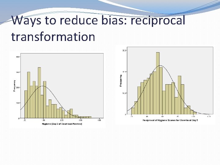
Ways to reduce bias: reciprocal transformation

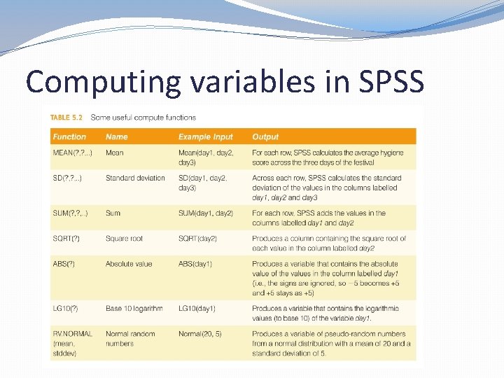
Computing variables in SPSS

Internal and External Validity

Internal validity

Internal validity �Given experimental design, can we determine that changes in the IV caused changes in the DV?

Causality �Experiment: involves manipulating one variable (the independent variable) to examine whether this change influences another variable (the dependent variable) �Example: manipulate presence of music to determine whether music affects job performance �Experiments often done to determine causality �Cause: one variable leads to changes in another variable �Example: listening to music causes job performance to improve

Causality �Causal relationship exists if: �Cause preceded effect �Cause related to (covaries with) effect �No plausible alternative explanations for effect other than cause

Causality �In experiments, this translates to: �Manipulating presumed cause (IV) to observe outcome (DV change/differences) � Some participants listen to music while working, some don’t �Evaluating whether variation in cause (IV) related to variation in effect (DV) � Does presence of music relate to job performance? What correlation exists? �Use good experimental design to control for other things that could lead to effect other than proposed cause � Randomly assign to music/no music conditions to control for confounding variables like experience, skill, age, etc. � Homogenous sample/representative of the population

Causality �Correlation does not prove causality �Can’t determine which variable came first � Did high job satisfaction lead to high job performance, or did high job performance lead to high job satisfaction �Relationship between 2 variables could be due to confound (third variable) � Possible that relationship between job satisfaction and job performance due to 3 rd variable, such as conscientiousness or salary

Causality �Manipulable cause �Things that can be varied by the experimenter: noise, lighting, medication dosage, training delivery method, etc. �Non-manipulable cause �Individual attributes: personality, gender, abilities, etc. �Events: exposure to workplace violence, past drug abuse �Experiments focus on manipulable causes �Non-manipulable causes may be measured so that they can be accounted/controlled for

Causality �Causal description: describing results of deliberately manipulating IV �Experiments are useful for this �Example: manipulating medication dosage levels to evaluate effect on anxiety �Causal explanation: determining why causal mechanism works the way it does �Experiments less useful for this �Example: why does medication dosage affect anxiety, and under what conditions does this medication work?

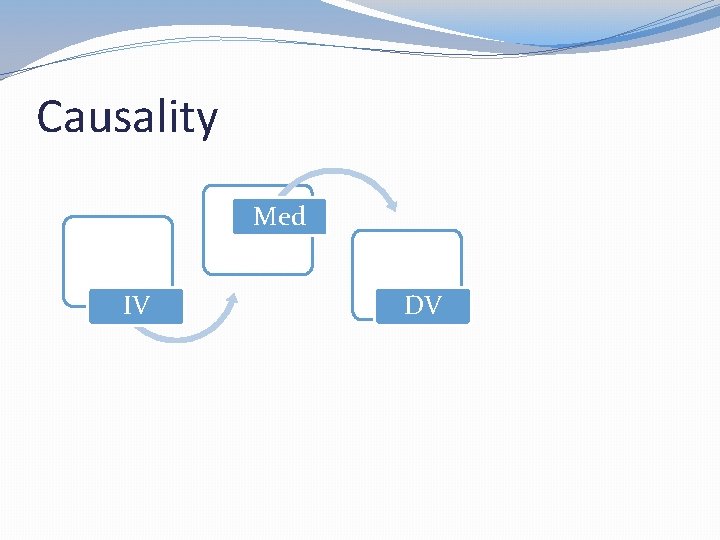
Causality �Moderator variables: explain under what conditions IV-DV relationship holds �Is relationship between music and performance different for highly-skilled workers than it is for entrylevel workers? �Mediator variables: explain mechanisms/processes by which IV affects DV �Those who listen to music are less bored, which improves job performance �Both can be useful in examining causal relationships

Causality Med IV DV

Validity �Validity: truth/correctness of inference �Cognitive behavioral therapy reduces depression �Threats to validity: reasons why inference might be incorrect �What if all participants in study were high SES women? �What if random assignment to conditions wasn’t done and those in treatment group had lower depression to begin with?

Internal validity �Threats to internal validity �Ambiguous temporal precedence �Selection �History �Maturation �Regression �Attrition �Testing �Instrumentation

Internal validity �Ambiguous temporal precedence �Not clear which way direction of causality flows � Does job performance lead to job satisfaction, or vice versa? � Shortcoming of correlational designs � Longitudinal designs can help with this �Reciprocal (bidirectional) relationships: A leads to B, which leads back to A � Example: Criminal behavior leads to incarceration, which leads to later criminal behavior

Internal validity �Selection �Participants differ in important ways across conditions before IV manipulation occurs �Example: individuals who volunteered for experimental leadership training program were motivated and extraverted than those who didn’t volunteer �Random assignment to conditions helps control for this

Internal validity �History=all events that happen between beginning of study and end of study that could have produced observed outcome in absence of IV manipulation �Example: While testing intervention to increase organizational commitment, location serving as experimental group institutes across-the-board pay raises �Can be reduced by selecting groups from same location and ensure that groups are tested at approximately the same time

Internal validity �Maturation=natural changes that would have occurred in absence of treatment � Physical changes � Cultural/economic changes �Example: children improve reading ability over time due to cognitive growth; this occurs with or without special reading programs �Can be reduced by ensuring participants same age, and from approximately same location

Internal validity �Regression artifacts �An extreme score on one occasion usually followed by less extreme score later � Example: Someone who receives high cognitive ability score less likely to receive this same score the next time � Very high/very low scores less probable; have more random error �Problematic when people placed into groups based on scores: regression to mean can mimic treatment effect � Example: individuals who scored highest on measure of depression chosen to participate in clinical trial for new depression drug �Randomly assign extreme scorers to conditions

Internal validity �Attrition (aka experimental mortality) �Not all participants complete the experiment �If attrition different across groups, can lead to incorrect conclusions � Example: In study of job retraining program, what if the individuals with lower cognitive ability dropped out of the treatment group (i. e. , the training) but not the control group? �Can’t be controlled by random assignment �Evaluate attrition post-hoc to determine if it threatens internal validity

Internal validity �Instrumentation �Instruments can change over time, which may look like treatment effect � Example: SAT scores have to be re-calibrated occasionally because average scores increase over time �Meaning of variable can also change over time � Example: Has the idea of work-life balance changed over time due to things like increased telecommuting and flextime? �Need to evaluate equivalence of measure over period of study � CFA and IRT-based approaches to measurement equivalence: is instrument measuring the same thing now that it was in the beginning of the study?

External validity

External validity �External validity: extent to which causal relationship holds over variations in persons, settings, treatments, and outcomes �Does it hold across variations included in study? �Does it hold across variations not included in study? �Targets of generalization: �Narrow to broad: VSU students to all college students �Broad to narrow: VSU students to single student �At similar level: VSU students to Georgia Southern students

External validity �Questions of external validity have to be assessed across multiple studies �Does same relationship hold across settings, participants, methods, outcomes? �Meta-analysis: statistically combines results of multiple studies �Can look at moderators (way constructs measured, participants, settings, etc. ) to determine if they affect IV -DV relationship

External validity �Population external validity: does sample represent target population? �Example: does sample of 200 fast-food employees in Florida generalize to population of fast-food employees in the US? �Ecological external validity: do conditions, settings, procedures, and other features of the experiment represent the real world? �Will results of experiment generalize to the real world? �Example: Do findings about submarine crew communication obtained using simulations apply to actual submarine crews during underwater emergency?

Sampling and external validity �Sample selected plays big role in external validity �Sample should reflect population that you’re trying to study �Results obtained using poor sample may not generalize to other settings �Example: Results of study using 20 severely depressed participants may not generalize to all individuals with diagnosed depression

Sampling basics �Theoretical/target population: all participants of interest to the researcher �Example: all autistic children in the U. S. �Nearly impossible to collect data from entire population �Accessible population (sampling frame): group of individuals the researcher has access to �Example: all autistic children in Lowndes county �Selected sample: individuals in accessible population who are asked to participate

Sampling basics �Sampling design: process used to select sample �Probability sampling: every individual in the population has a known and non-zero chance of being chosen to participate �Non-probability sampling: no way of determining probability of any one person in the population being chosen �Sampling bias likely

Probability sampling �Simple random sampling: all individuals in population have an equal chance of being included in the sample �Example: Population is all VSU students: all students listed and assigned a random number. All participants with a “ 5” at the end of their number chosen to participate �Very time consuming �Difficult, if not impossible, to create list of whole population

Probability sampling �Stratified random sampling: divide population into groups (strata) based on variable of interest (age, race, occupation, etc. ) and randomly sample within each strata �Helps ensure sample representative of population �Can take proportion of population each strata represents into account when selecting sample �Variable(s) used to create strata should be theoretically relevant �Example: VSU students divided into 2 groups (grad students and undergrad students), and random sampling done within each group

Probability sampling �Cluster sampling: unit of sampling is the group, rather than the individual-groups are randomly sampled �Cluster: non-overlapping groups of individuals (K-12 schools, biotech companies, Red Cross chapters, etc. ) �Create list of clusters, randomly sample clusters, and then either select all or randomly sample from each chosen cluster �Useful when a list of all individuals in population can’t be created �Example: Create list of all universities with graduate psychology programs in the U. S. , randomly select 15 universities, and then sample all individuals in the

Nonprobability sampling �Quota sampling: set quotas for the number of participants in certain subgroups (age, sex, race, etc. ) and haphazardly select participants until quota is met �Example: Need 70 VSU undergrads and 30 VSU grad students, so sit out by the library and ask students to take a survey until both quotas have been met

Nonprobability sampling �Convenience sampling: sampling that does not try to determine sample characteristics beforehand �Convenience/Accidental sampling: Researcher gets participants however they can � Example: Researcher gives survey to all of their classmates, friends, and family members � Things like SONA and Mechanical. Turk are also convenience sampling �Snowball sampling: Have your participants help in the sampling process by having them suggest other participants who could participate in your study � Good if you’re studying a small population (like CEOs) and don’t know how to find more participants

Threats to external validity �Interaction of causal relationship with units �Interaction of causal relationship over treatment conditions �Interaction of causal relationship with outcomes �Interaction of causal relationship with settings �Context-dependent mediation

Threats to external validity �Interaction of causal relationship with units: effect found with some participants doesn’t hold across other participants �Example: findings of a relationship between computer adaptive training and improved post-test performance might hold for college students, but not for older adults in the workplace who are less computer savvy

Threats to external validity �Interaction of causal relationship over treatment variations: effect found with one treatment variation might not hold with other variations of treatment �Example: new leadership training program is effective in improving subordinate ratings of leadership if implemented by highly skilled trainers, but not at all effective if implemented by novice trainers

Threats to external validity �Interaction of causal relationship with outcomes: effect on one kind of outcome observation may not hold if other outcome observations were used �Example: new leadership training program leads to increased ratings of performance from subordinates, but not from supervisors

Threats to external validity �Interaction of causal relationship with settings: effect found in one setting may not hold if other settings used �Example: strong relationship between test instructions and faking in research settings, but not in high-stakes selection settings

Threats to external validity �Context-dependent mediation: mediator of causal relationship in one context may not mediate in another context �Example: What if quality of communication mediates the relationship between emotional intelligence and team viability for newly-formed virtual teams, but not for virtual teams that have been working together for 6 months or longer?

Is there evidence of external validity? �Usually consider constancy of causal direction (effect always goes the same way) as evidence of generalizability, thus external validity �Differences in size of effect important to consider

Correlation and regression

Associational research �Looks at the relationship between two variables �Usually continuous variables �No manipulation of IV �Correlation coefficient shows relationship between 2 variables �Regression: equation used to predict outcome value based on predictor value �Multiple regression: same, but uses more than 1 predictor

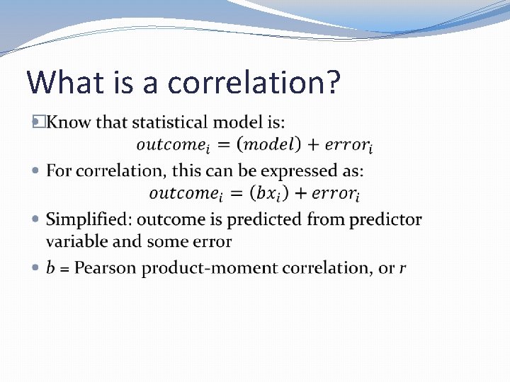
What is a correlation? �

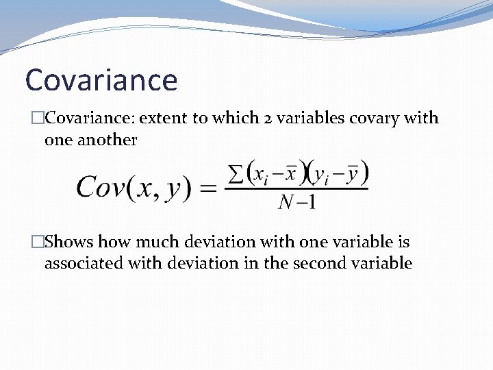
Covariance �Covariance: extent to which 2 variables covary with one another �Shows how much deviation with one variable is associated with deviation in the second variable

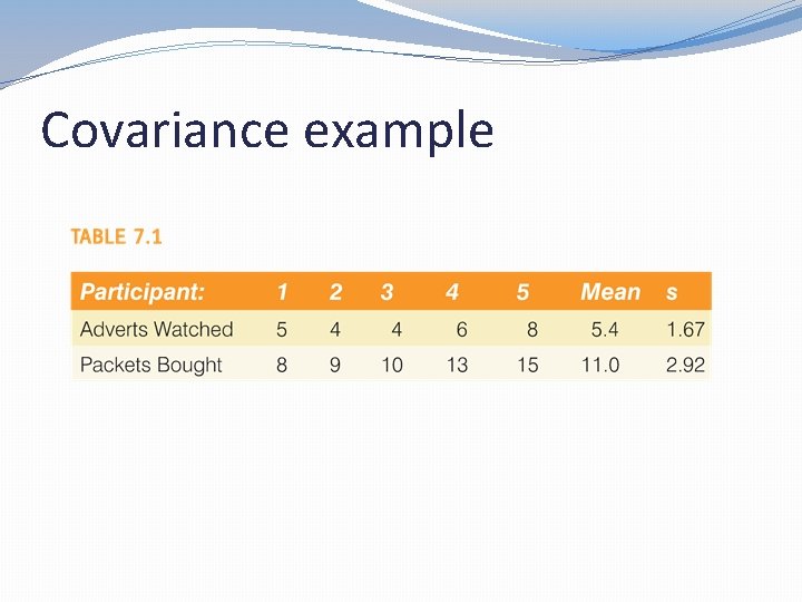
Covariance example

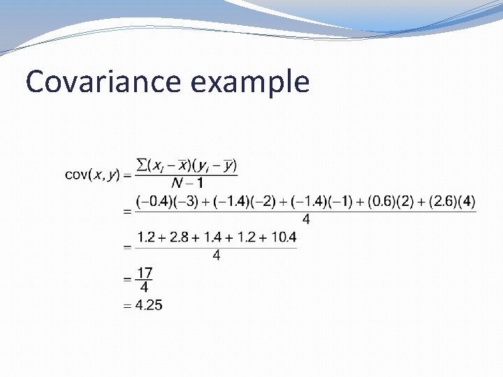
Covariance example

Covariance �Positive covariance: As one variable deviates from mean, other variable deviates in same direction �Negative covariance: As one variable deviates from mean, other variable deviates in opposite direction �Problem with covariance: depends on scales variables measured on �Can’t be compared across measures �Need standardized covariance to compare across measures

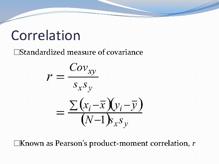
Correlation �Standardized measure of covariance �Known as Pearson’s product-moment correlation, r

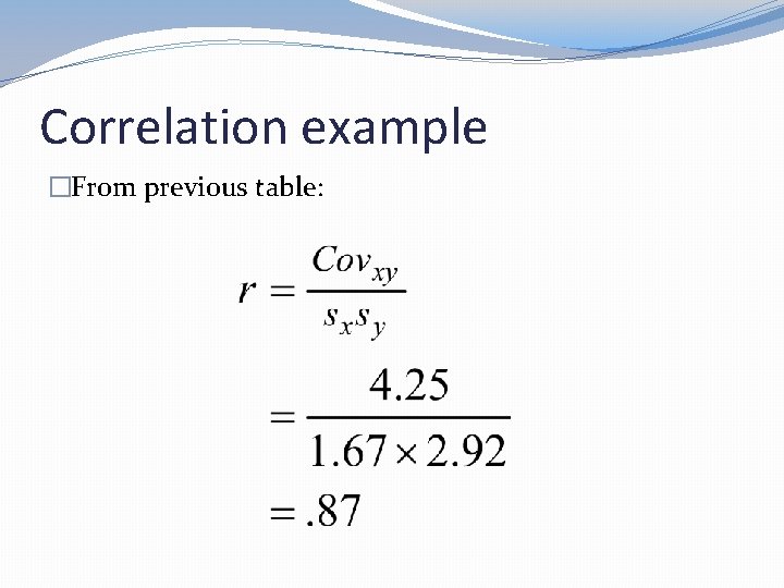
Correlation example �From previous table:

Correlation �Values range from -1 to +1 �+1: perfect positive correlation: as one variable increases, other increases by proportionate amount �-1: perfect negative correlation: as one variable increases, other decreases by proportionate amount � 0: no relationship. As one variable changes, other stays the same

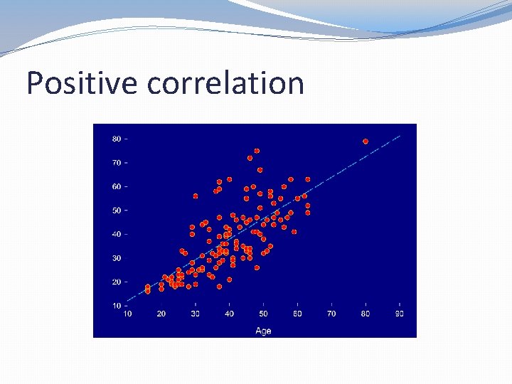
Positive correlation

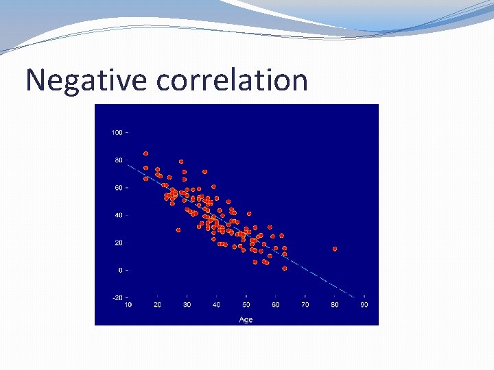
Negative correlation

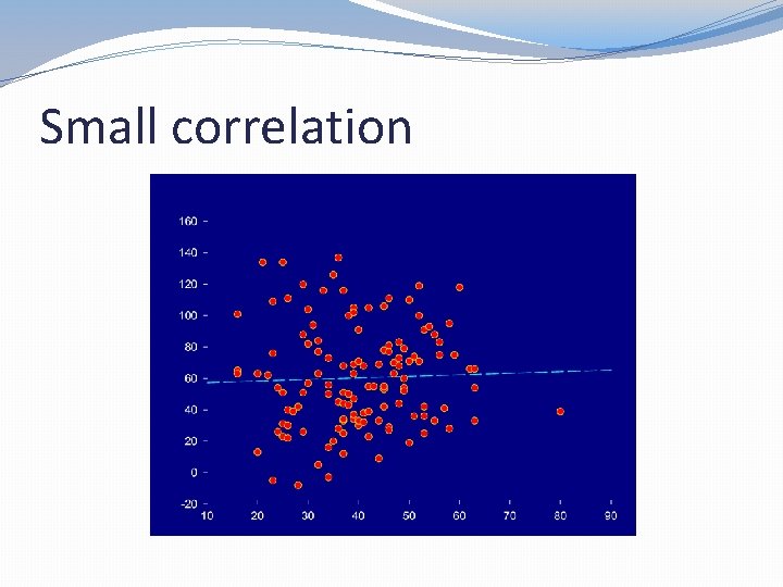
Small correlation

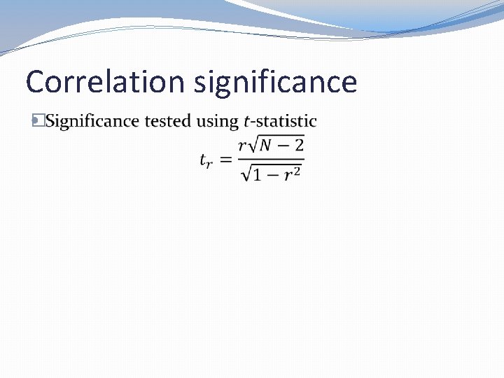
Correlation significance �

Correlation and causality �Correlation DOES NOT imply causality!!! �Only shows us that 2 variables are related to one another �Why correlation doesn’t show causality: � 3 rd variable problem: some other variable (not measured) responsible for observed relationship �No way to determine directionality: does a cause b, or does b cause a?

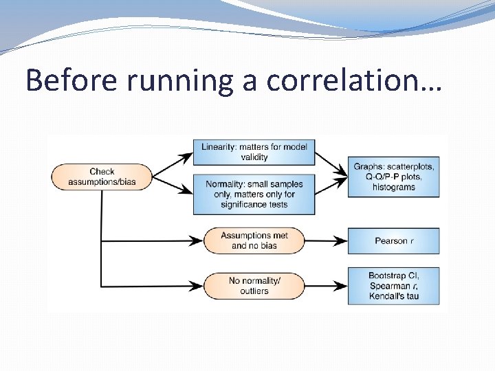
Before running a correlation…

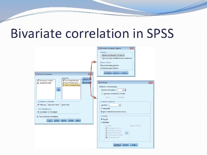
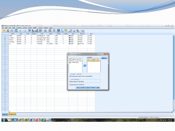
Bivariate correlation in SPSS

Note on pairwise & listwise deletion �Pairwise deletion: removes cases from analysis on an analysis-by-analysis basis � 3 variables: A, B, & C � Correlation matrix between A, B, & C � Case 3 is missing data on variable B, but not on A or C � Case 3 will be excluded from correlation between B & C, and A & B, but not from correlation beteween A & C �Advantage: keep more of your data �Disadvantage: not all analyses will include the same cases: can bias results

Note on pairwise & listwise deletion �Listwise deletion: removes cases from analysis if they are missing data on any variable under consideration � 3 variables: A, B, & C � Correlation matrix between A, B, & C � Case 3 is missing data on variable B, but not on A or C � Case 3 will be excluded from correlation between B & C, A & B, and A & C �Advantage: less prone to bias �Disadvantage: don’t get to keep as much data �Usually a better option than pairwise

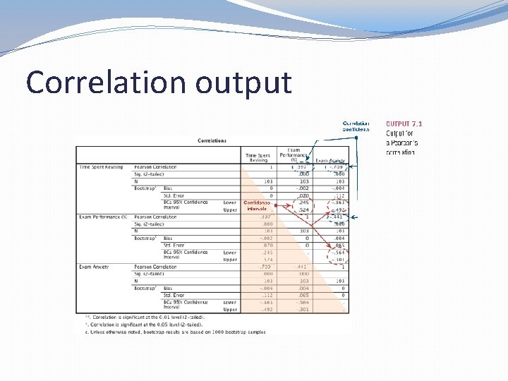
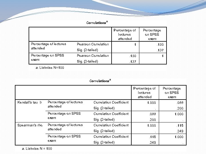
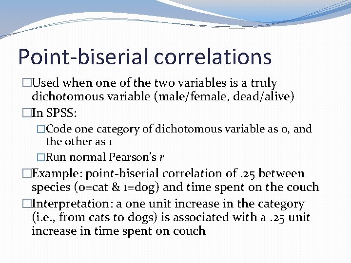
Correlation output

Interpreting correlations �Look at statistical significance �Also, look at size of correlation: �+/-. 10: small correlation �+/-. 30: medium correlation �+/-. 50: large correlation

Coefficient of determination, 2 R �Amount of variance in one variable shared by other variable �Example: pretend R 2 between cognitive ability and job performance is. 25 �Interpretation: 25% of variance in cognitive ability shared by variance in job performance �Slightly incorrect but easier way to think of it: 25% of the variance in job performance is accounted for by cognitive ability

Spearman’s correlation coefficient �Also called Spearman’s rho (ρ) �Non-parametric �Based on ranked, not interval or ratio, data �Good for minimizing effect of outliers and getting around normality issues �Ranks data (lowest to highest score) �Then, uses Pearson’s r formula on ranked data

Kendall’s tau (τ) �Non-parametric correlation �Also ranks data �Better than Spearman’s rho if: �Small data set �Large number of tied ranks �More accurate representation of correlation in population than Spearman’s rho

Point-biserial correlations �Used when one of the two variables is a truly dichotomous variable (male/female, dead/alive) �In SPSS: �Code one category of dichotomous variable as 0, and the other as 1 �Run normal Pearson’s r �Example: point-biserial correlation of. 25 between species (0=cat & 1=dog) and time spent on the couch �Interpretation: a one unit increase in the category (i. e. , from cats to dogs) is associated with a. 25 unit increase in time spent on couch

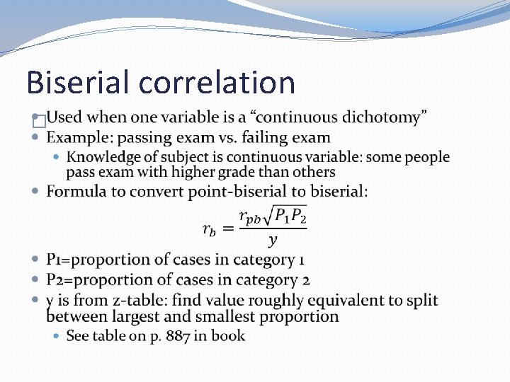
Biserial correlation �

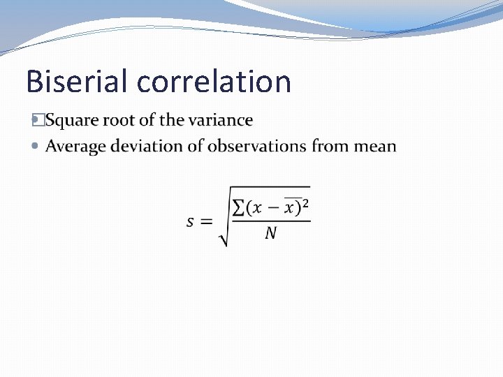
Biserial correlation �

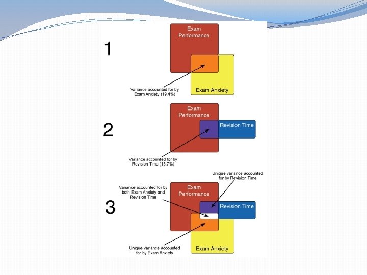
Partial correlation �Correlation between two variables when the effect of a third variable has been held constant �Controls for effect of third variable on both variables �Rationale: if third variable correlated (shares variance) with 2 variables of interest, correlation between these 2 variables won’t be accurate unless effect of 3 rd variable is controlled for

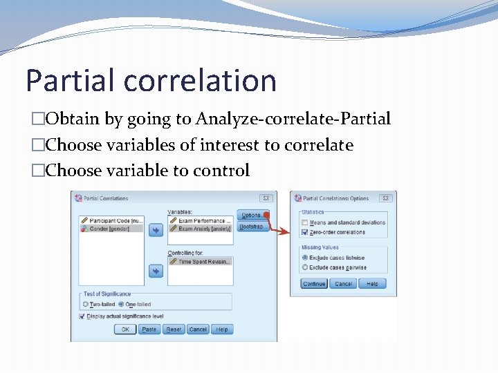
Partial correlation �Obtain by going to Analyze-correlate-Partial �Choose variables of interest to correlate �Choose variable to control

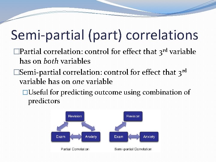
Semi-partial (part) correlations �Partial correlation: control for effect that 3 rd variable has on both variables �Semi-partial correlation: control for effect that 3 rd variable has on one variable �Useful for predicting outcome using combination of predictors

Calculating effect size �Can square Pearson’s correlation to get R 2: proportion of variance shared by variables �Can also square Spearman’s rho to get R 2 s: proportion of variance in ranks shared by variables �Can’t square Kendall’s tau to get proportion of variance shared by variables

Regression �

Regression �

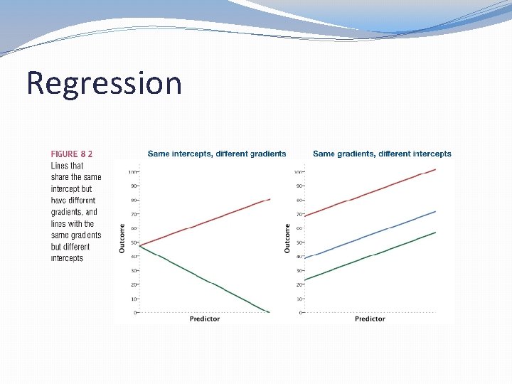
Regression

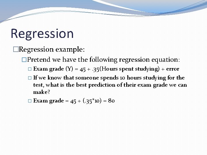
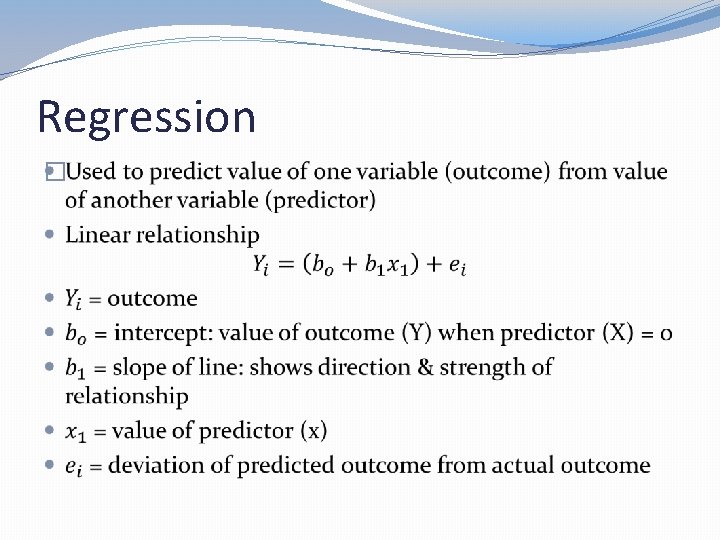
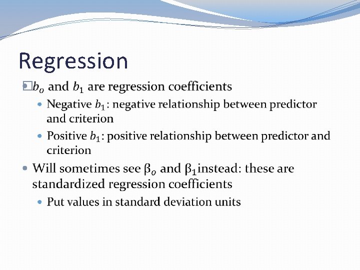
Regression �Regression example: �Pretend we have the following regression equation: � Exam grade (Y) = 45 +. 35(Hours spent studying) + error � If we know that someone spends 10 hours studying for the test, what is the best prediction of their exam grade we can make? � Exam grade = 45 + (. 35*10) = 80

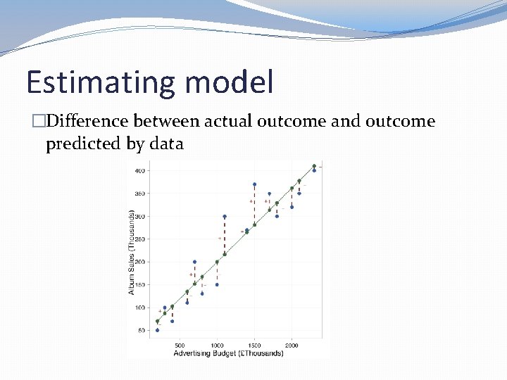
Estimating model �Difference between actual outcome and outcome predicted by data

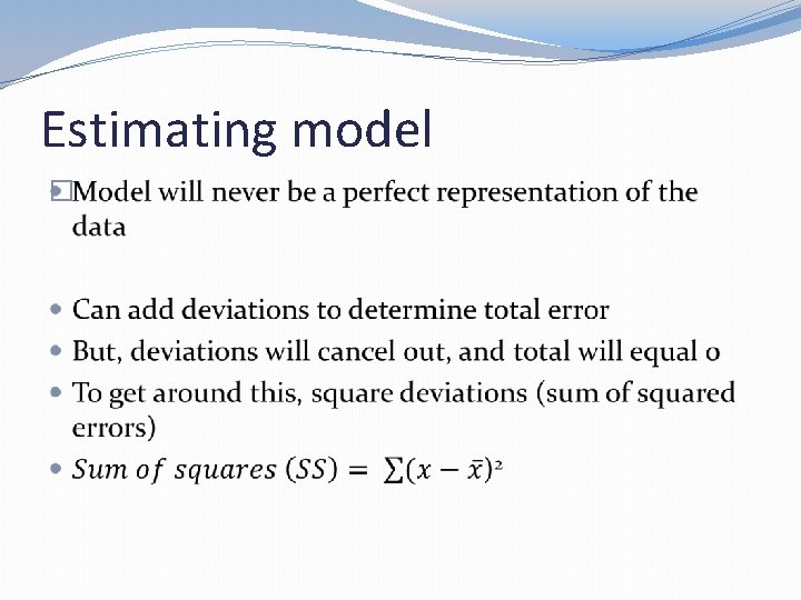
Estimating model �

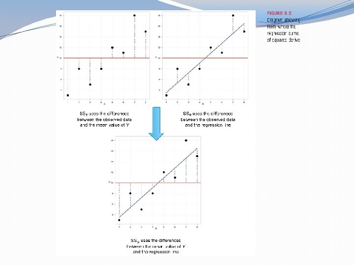
Estimating model �Total sum of squares (SST): Total sum of squared differences between observed data and mean value of Y �Model sum of squares (SSM): Improvement in prediction as result of using regression model rather than mean

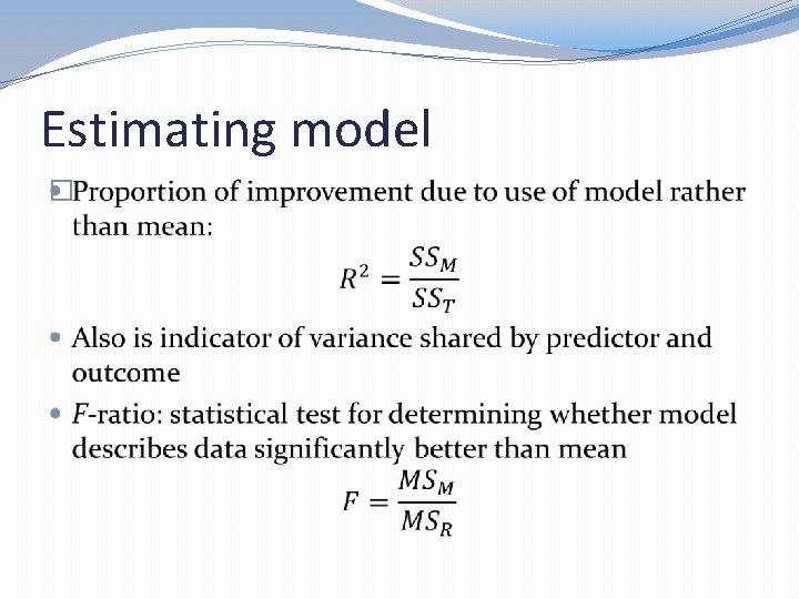
Estimating model �

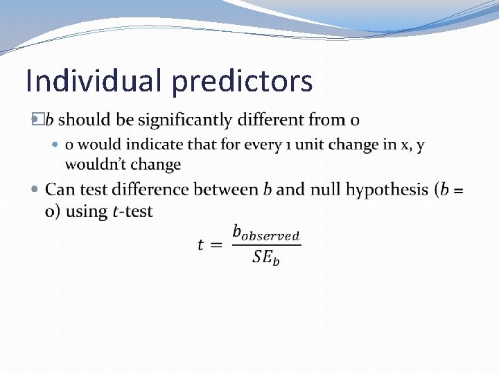
Individual predictors �