Introduction to Statistical Models and Factoring l l

Introduction to Statistical Models and Factoring l l l dependent and independent models “traditional” and possible applications of independent models 3 -way sampling problem

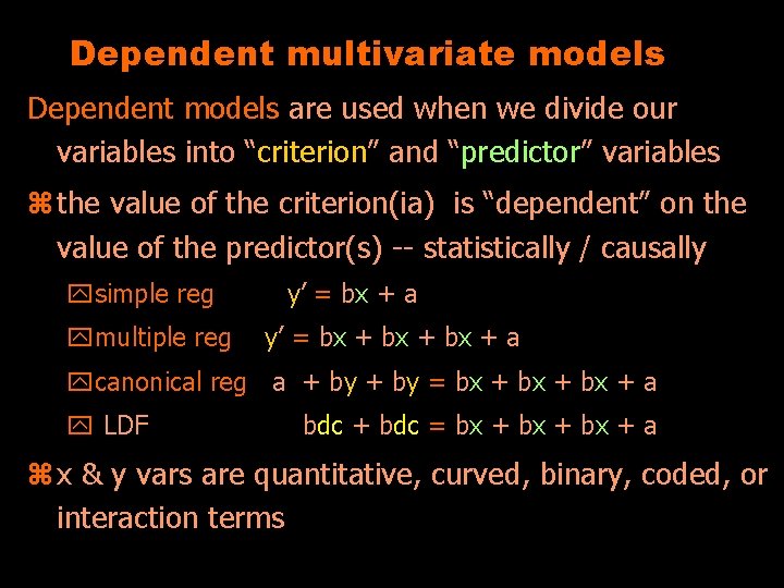
Dependent multivariate models Dependent models are used when we divide our variables into “criterion” and “predictor” variables z the value of the criterion(ia) is “dependent” on the value of the predictor(s) -- statistically / causally ysimple reg ymultiple reg y’ = bx + a y’ = bx + a ycanonical reg a + by = bx + a y LDF bdc + bdc = bx + a z x & y vars are quantitative, curved, binary, coded, or interaction terms

Dependent multivariate models, cont. Dependent models … z these are the General Linear Models from “multivariate class” z research questions/hypotheses are about which predictors (with what weightings) are useful for estimating what criteria

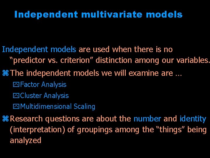
Independent multivariate models Independent models are used when there is no “predictor vs. criterion” distinction among our variables. z The independent models we will examine are … y. Factor Analysis y. Cluster Analysis y. Multidimensional Scaling z Research questions are about the number and identity (interpretation) of groupings among the “things” being analyzed

Independent multivariate models: “Traditional” Uses z Factor variables to find the number and identity of the different kinds of information Factor the 25 questions from client’s intake interviews z Cluster people to find the number and identity of the different kinds of characteristic profiles Cluster 250 students to took a standardized test z Scale stimuli to find the “rules of stimulus similarity and dissimilarity” MDscale 24 shape stimuli Before we get into the “alternative” uses of these models. . .

3 -way sampling problem z from a statistical or research design perspective “sampling” usually refers to the selection of some set of people from which data will be collected, for the purposes of representing what the results would be if data were collected from the entire population of people in which the researcher is interested z from a psychometric perspective “sampling” is a broader issue, with three dimensions ysampling respondents to represent the desired population of individuals ysampling attributes to represent some desired domain of characteristics ysampling stimuli (things or people) to represent the desired category(ies) of objects

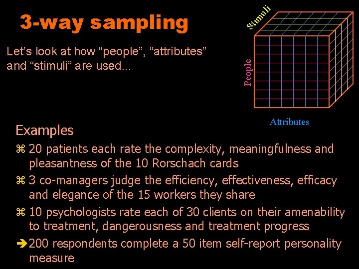
Let’s look at how “people”, “attributes” and “stimuli” are used. . . Examples im ul i St People 3 -way sampling Attributes z 20 patients each rate the complexity, meaningfulness and pleasantness of the 10 Rorschach cards z 3 co-managers judge the efficiency, effectiveness, efficacy and elegance of the 15 workers they share z 10 psychologists rate each of 30 clients on their amenability to treatment, dangerousness and treatment progress è 200 respondents complete a 50 item self-report personality measure

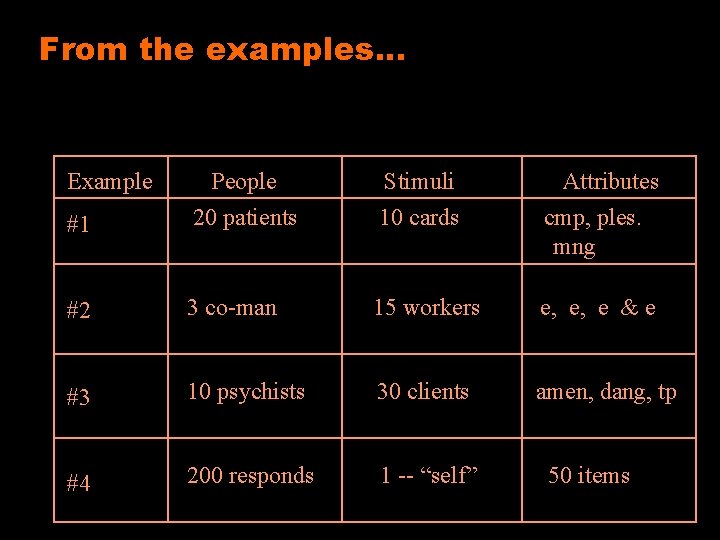
From the examples. . . Example #1 People 20 patients Stimuli 10 cards Attributes cmp, ples. mng #2 3 co-man 15 workers e, e, e & e #3 10 psychists 30 clients amen, dang, tp #4 200 responds 1 -- “self” 50 items

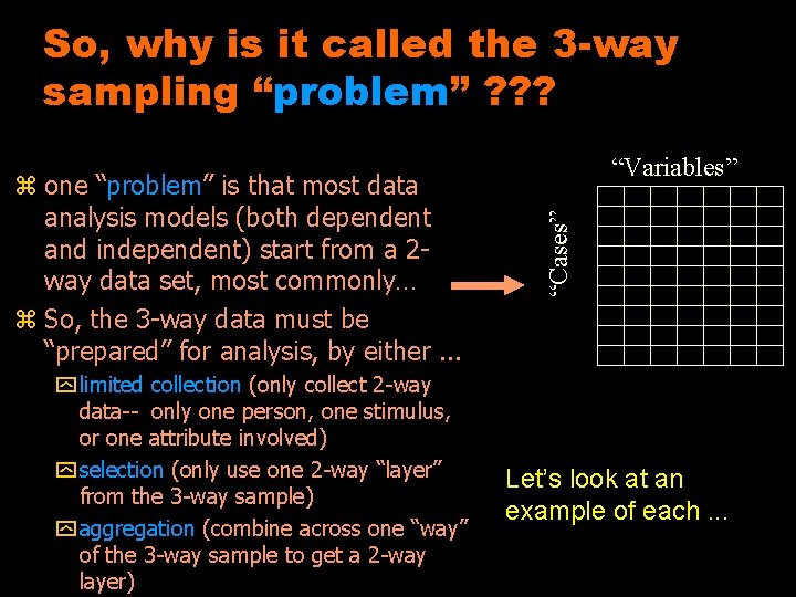
So, why is it called the 3 -way sampling “problem” ? ? ? y limited collection (only collect 2 -way data-- only one person, one stimulus, or one attribute involved) y selection (only use one 2 -way “layer” from the 3 -way sample) y aggregation (combine across one “way” of the 3 -way sample to get a 2 -way layer) “Cases” z one “problem” is that most data analysis models (both dependent and independent) start from a 2 way data set, most commonly… z So, the 3 -way data must be “prepared” for analysis, by either. . . “Variables” Let’s look at an example of each. . .

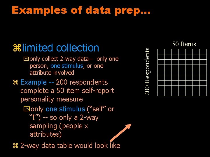
Examples of data prep. . . y only collect 2 -way data-- only one person, one stimulus, or one attribute involved z Example -- 200 respondents complete a 50 item self-report personality measure yonly one stimulus (“self” or “I”) -- so only a 2 -way sampling (people x attributes) z 2 -way data table would look like 200 Respondents zlimited collection 50 Items

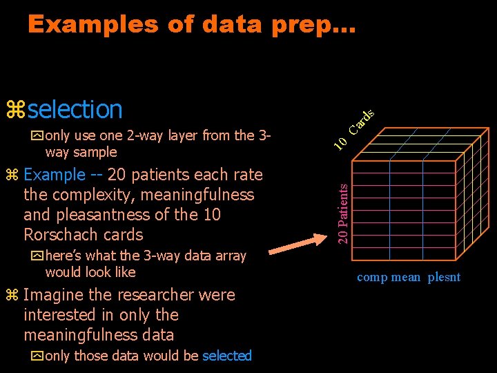
Examples of data prep. . . z Example -- 20 patients each rate the complexity, meaningfulness and pleasantness of the 10 Rorschach cards y here’s what the 3 -way data array would look like z Imagine the researcher were interested in only the meaningfulness data y only those data would be selected rd Ca 10 20 Patients y only use one 2 -way layer from the 3 way sample s zselection comp mean plesnt

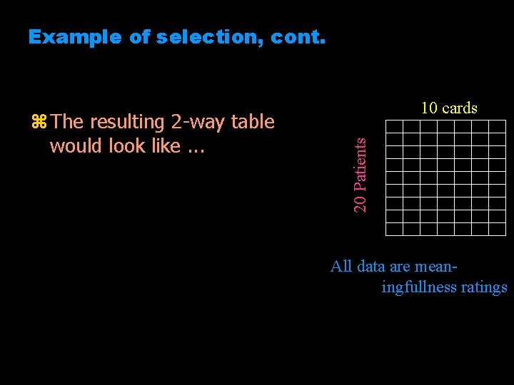
Example of selection, cont. 20 Patients z The resulting 2 -way table would look like. . . 10 cards All data are meaningfullness ratings

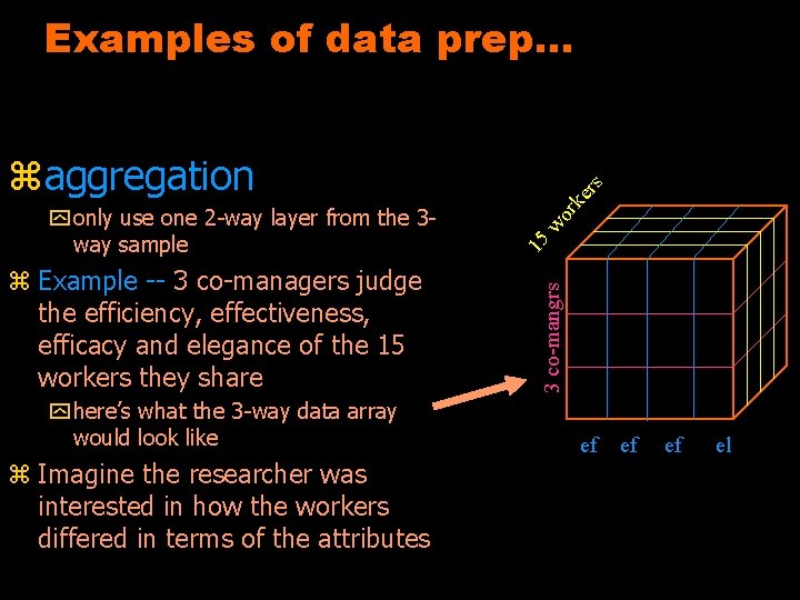
Examples of data prep. . . y here’s what the 3 -way data array would look like z Imagine the researcher was interested in how the workers differed in terms of the attributes er rk wo 3 co-mangrs z Example -- 3 co-managers judge the efficiency, effectiveness, efficacy and elegance of the 15 workers they share 15 y only use one 2 -way layer from the 3 way sample s zaggregation ef ef ef el

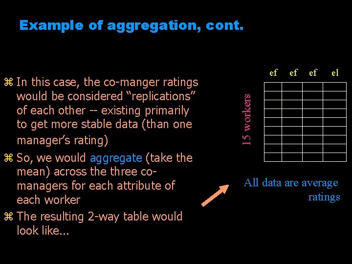
Example of aggregation, cont. ef ef el 15 workers z In this case, the co-manger ratings would be considered “replications” of each other -- existing primarily to get more stable data (than one manager’s rating) z So, we would aggregate (take the mean) across the three comanagers for each attribute of each worker z The resulting 2 -way table would look like. . . ef All data are average ratings

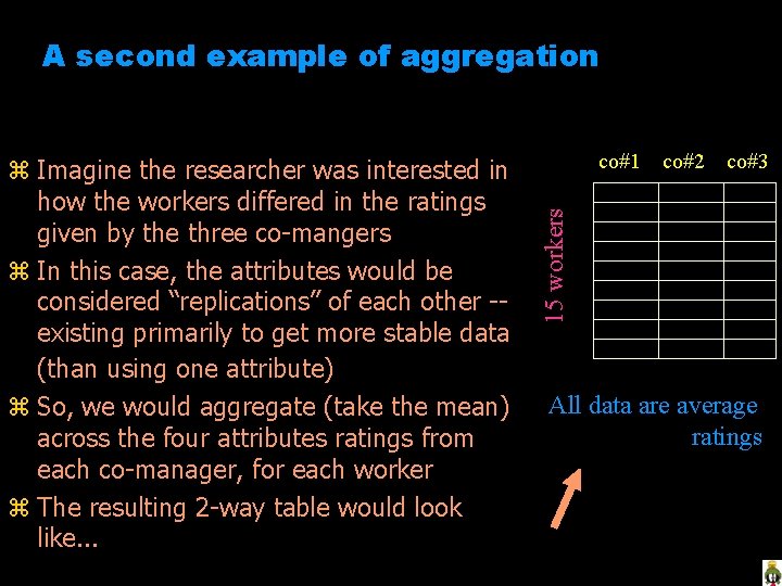
A second example of aggregation co#1 co#2 co#3 15 workers z Imagine the researcher was interested in how the workers differed in the ratings given by the three co-mangers z In this case, the attributes would be considered “replications” of each other -existing primarily to get more stable data (than using one attribute) z So, we would aggregate (take the mean) across the four attributes ratings from each co-manager, for each worker z The resulting 2 -way table would look like. . . All data are average ratings

Different ways of treating data for the different models z The 2 -way data table we have been discussing is often labeled the “X” matrix z starting with “X”, different things are done to prepare the data for different model z Let’s look at these. . z Remember, we’ll start with the “traditional” uses of the different models, and then look at the different ways they can be used

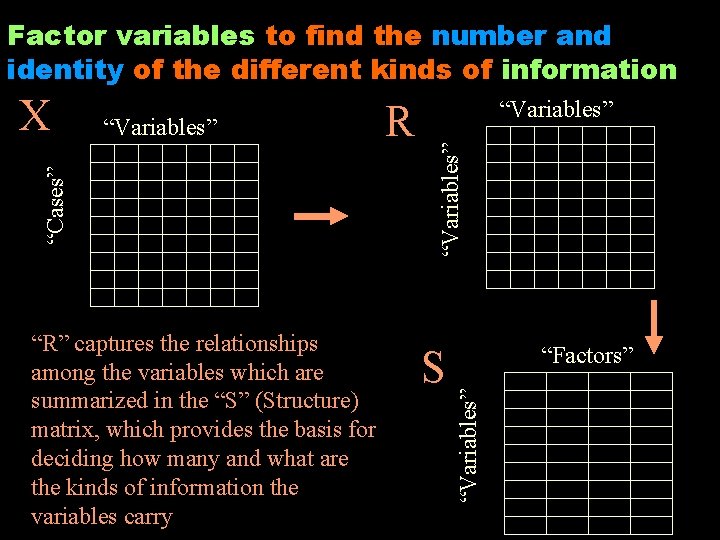
Factor variables to find the number and identity of the different kinds of information S “Factors” “Variables” “R” captures the relationships among the variables which are summarized in the “S” (Structure) matrix, which provides the basis for deciding how many and what are the kinds of information the variables carry R “Variables” “Cases” X

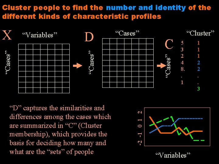
Cluster people to find the number and identity of the different kinds of characteristic profiles D “Cases” “D” captures the similarities and differences among the cases which are summarized in “C” (Cluster membership), which provides the basis for deciding how many and what are the “sets” of people “Cases” C “Cluster” 5 3 2 4 8. . 1 -2 -1 0 1 2 “Variables” “Cases” X “Variables” 1 1 1 2 2. . 3

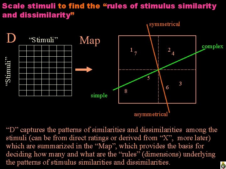
Scale stimuli to find the “rules of stimulus similarity and dissimilarity” symmetrical D “Stimuli” Map “Stimuli” 1 2 7 5 simple 8 6 complex 4 3 asymmetrical “D” captures the patterns of similarities and dissimilarities among the stimuli (can be from direct ratings or derived from “X”, more later) which are summarized in the “Map”, which provides the basis for deciding how many and what are the “rules” (dimensions) underlying the patterns of stimulus similarities and dissimilarities.

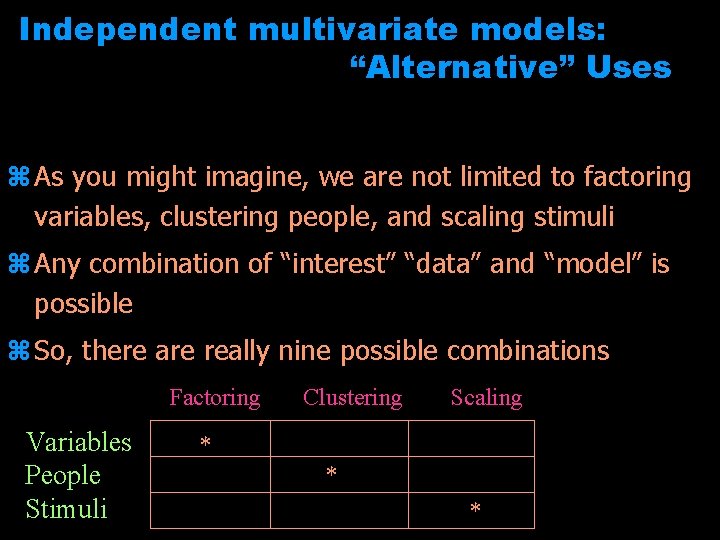
Independent multivariate models: “Alternative” Uses z As you might imagine, we are not limited to factoring variables, clustering people, and scaling stimuli z Any combination of “interest” “data” and “model” is possible z So, there are really nine possible combinations Factoring Variables People Stimuli Clustering Scaling * * *

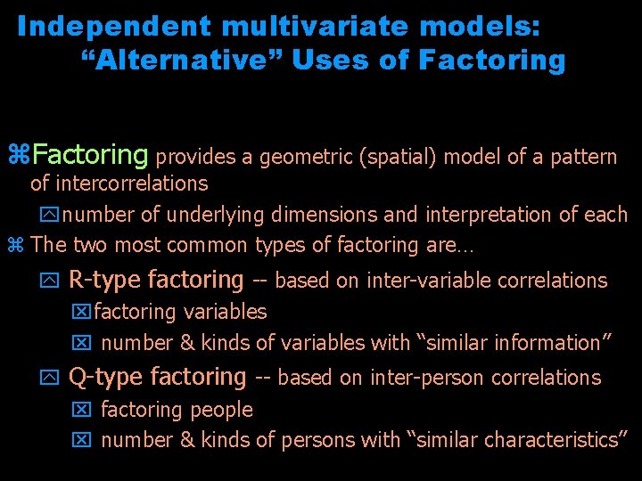
Independent multivariate models: “Alternative” Uses of Factoring z. Factoring provides a geometric (spatial) model of a pattern of intercorrelations ynumber of underlying dimensions and interpretation of each z The two most common types of factoring are… y R-type factoring -- based on inter-variable correlations xfactoring variables x number & kinds of variables with “similar information” y Q-type factoring -- based on inter-person correlations x factoring people x number & kinds of persons with “similar characteristics”

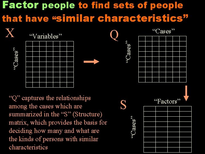
Factor people to find sets of people that have “similar characteristics” “Factors” S “Cases” “Q” captures the relationships among the cases which are summarized in the “S” (Structure) matrix, which provides the basis for deciding how many and what are the kinds of persons with similar characteristics Q “Cases” “Variables” “Cases” X

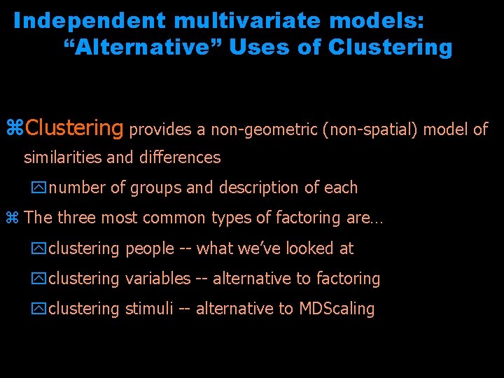
Independent multivariate models: “Alternative” Uses of Clustering z. Clustering provides a non-geometric (non-spatial) model of similarities and differences ynumber of groups and description of each z The three most common types of factoring are… yclustering people -- what we’ve looked at yclustering variables -- alternative to factoring yclustering stimuli -- alternative to MDScaling

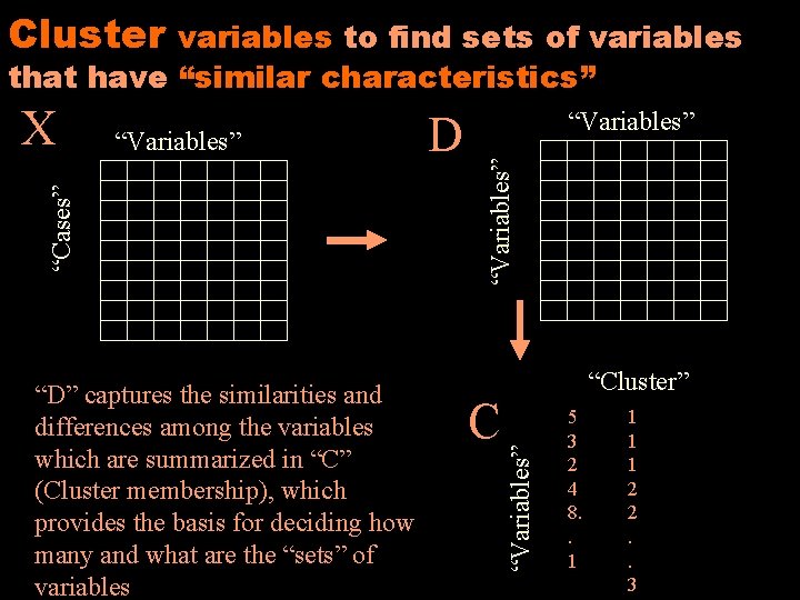
Cluster variables to find sets of variables that have “similar characteristics” C “Cluster” “Variables” “D” captures the similarities and differences among the variables which are summarized in “C” (Cluster membership), which provides the basis for deciding how many and what are the “sets” of variables D “Variables” “Cases” X 5 3 2 4 8. . 1 1 2 2. . 3

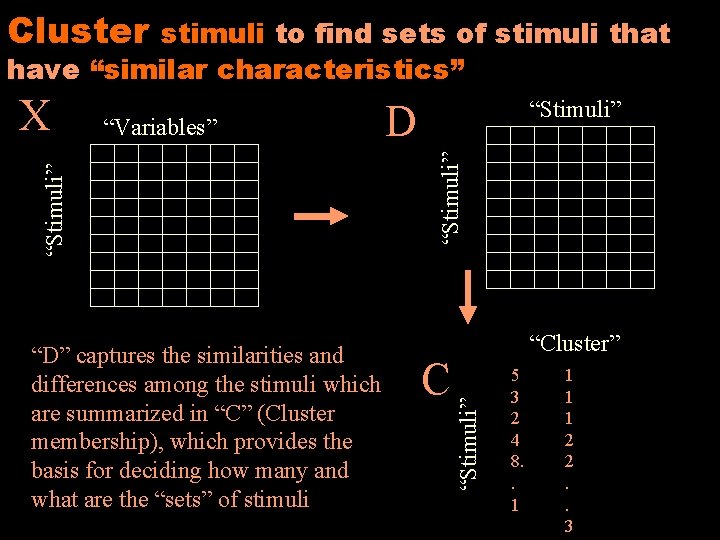
Cluster stimuli to find sets of stimuli that have “similar characteristics” D C “Cluster” “Stimuli” “D” captures the similarities and differences among the stimuli which are summarized in “C” (Cluster membership), which provides the basis for deciding how many and what are the “sets” of stimuli “Stimuli” “Variables” “Stimuli” X 5 3 2 4 8. . 1 1 2 2. . 3

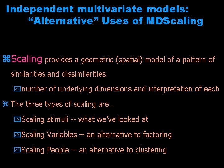
Independent multivariate models: “Alternative” Uses of MDScaling z. Scaling provides a geometric (spatial) model of a pattern of similarities and dissimilarities ynumber of underlying dimensions and interpretation of each z The three types of scaling are… y. Scaling stimuli -- what we’ve looked at y. Scaling Variables -- an alternative to factoring y. Scaling People -- an alternative to clustering

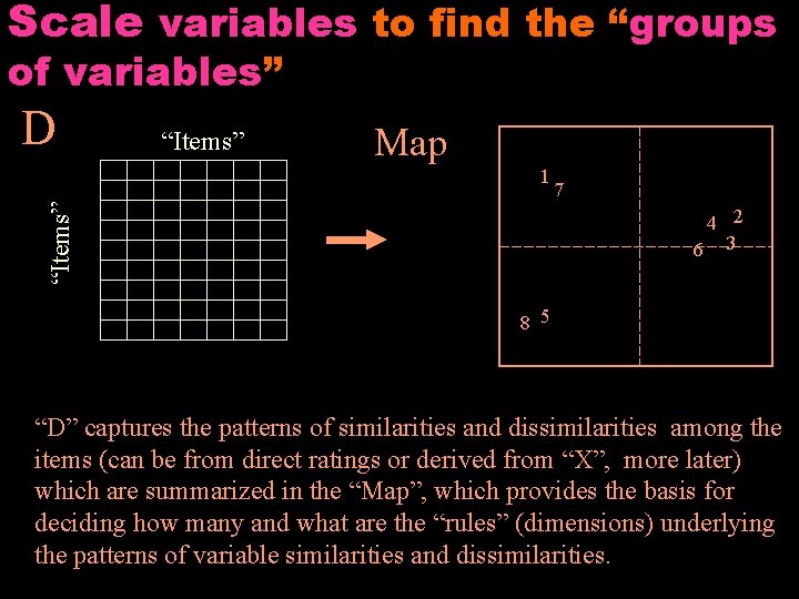
Scale variables to find the “groups of variables” D “Items” Map “Items” 1 7 4 2 6 3 8 5 “D” captures the patterns of similarities and dissimilarities among the items (can be from direct ratings or derived from “X”, more later) which are summarized in the “Map”, which provides the basis for deciding how many and what are the “rules” (dimensions) underlying the patterns of variable similarities and dissimilarities.

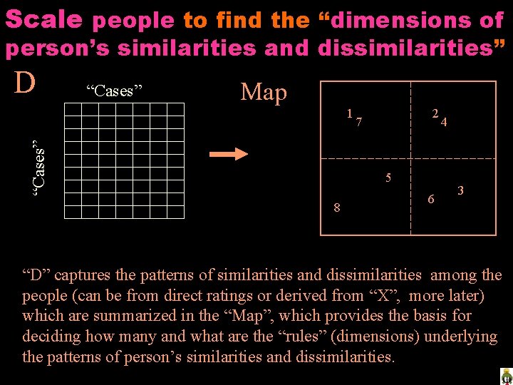
Scale people to find the “dimensions of person’s similarities and dissimilarities” D “Cases” Map “Cases” 1 2 7 5 8 6 4 3 “D” captures the patterns of similarities and dissimilarities among the people (can be from direct ratings or derived from “X”, more later) which are summarized in the “Map”, which provides the basis for deciding how many and what are the “rules” (dimensions) underlying the patterns of person’s similarities and dissimilarities.