Introduction to state space model and Kalman filter

Introduction to state space model and Kalman filter JEN-WEN LIN, PHD

Administrative items � Final exam � Friday August 14, 2015, 2 -4 pm, EX 200 � Practice questions have already posted on portal � TA tutorial session on Monday August 10, 2015, in class � Be ready for expressing a given model in terms of the state-space model representation �A detailed write-up for the state-space model and Kalman filter to post on portal latter � Office hours � Date: 13 -AUG-15 � Location: SS 1078 ( Sidney Smith Hall ) � Time: 11: 30 to 13: 00

Introduction to state-space model � State-space models, originally developed by control engineers (Kalman 1960), are useful tools for expressing dynamic systems that involve with unobserved state variables. � A state-space model consists of two equations: a transition equation (or state equation) and a measurement equation. � Measurement Equation: An equation that describes the relation between observed variables (data) and unobserved state variable. � Transition Equation: An equation that describes the dynamics of the state variables. The transition equation has the form of a firstorder difference equation in the state vector.

State space model � Measurement � Transition where equation

Example

Example

Introduction to Kalman filtering � Once a dynamic time series model is written as the state-space form, the Kalman filter is readily available for inference on the unobserved state vector betat, conditional on the parameters of the model and the appropriate information set. � For simpilicity, we shall introduce Kalman filtering using the regression with time-varying coefficients.

Some notations

Introduction to Kalman filtering � Prediction: At the beginning of time t, we may want to form an optimal predictor of yt based on all the available information up to time t-1, i. e. yt|t-1. Note that we need to know betat|t-1 to predict yt|t-1. � Updating: Once yt is realized at the end of time t, the prediction error can be calculated as etat|t-1=yt-yt|t-1. This prediction error contains new information about betat beyond that contained in betat|t-1. Thus, after observing yt, a more accurate inference can be made of betat|t, an inference of betat based on information up to time t, may be of the following form:

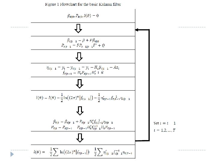
Mathematics for prediction and updating steps

MLE estimation and Kalman Filter

Smoothing step � Smoothing betat|T provides us with a more accurate inference on betat, since it uses more information than the basic filter. The following two equations can be iterated backwards for t=T-1, T-2, …, 1, to get the smoothed estimates.