INTRODUCTION TO STATA UCLA IDRE STATISTICAL CONSULTING GROUP

INTRODUCTION TO STATA UCLA IDRE STATISTICAL CONSULTING GROUP ANDY LIN FALL 2018

PURPOSE OF THE SEMINAR • This seminar introduces the usage of Stata for data analysis • Topics include • Stata as a data analysis software package • Navigating Stata • Data import • Exploring data • Data visualization • Data management • Basic statistical analysis

STATA

WHAT IS STATA? • Stata is an easy to use but very powerful data analysis software package • Stata offers a wide array of statistical tools that include both standard methods and newer, advanced methods, as new releases of Stata are distributed annually

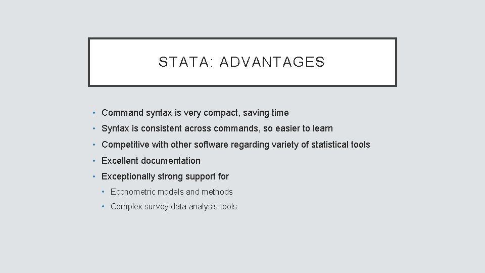
STATA: ADVANTAGES • Command syntax is very compact, saving time • Syntax is consistent across commands, so easier to learn • Competitive with other software regarding variety of statistical tools • Excellent documentation • Exceptionally strong support for • Econometric models and methods • Complex survey data analysis tools

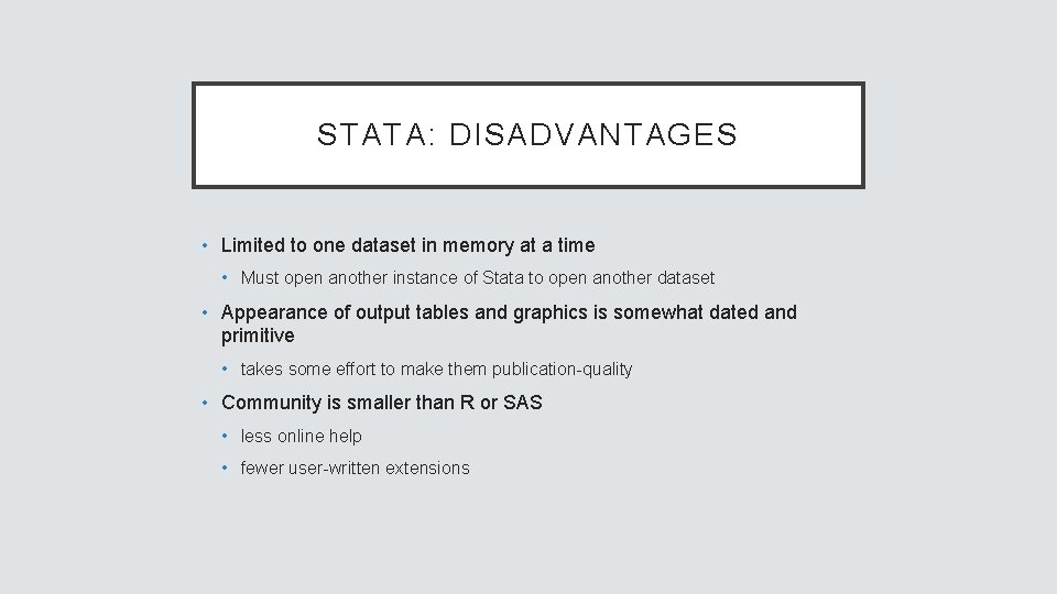
STATA: DISADVANTAGES • Limited to one dataset in memory at a time • Must open another instance of Stata to open another dataset • Appearance of output tables and graphics is somewhat dated and primitive • takes some effort to make them publication-quality • Community is smaller than R or SAS • less online help • fewer user-written extensions

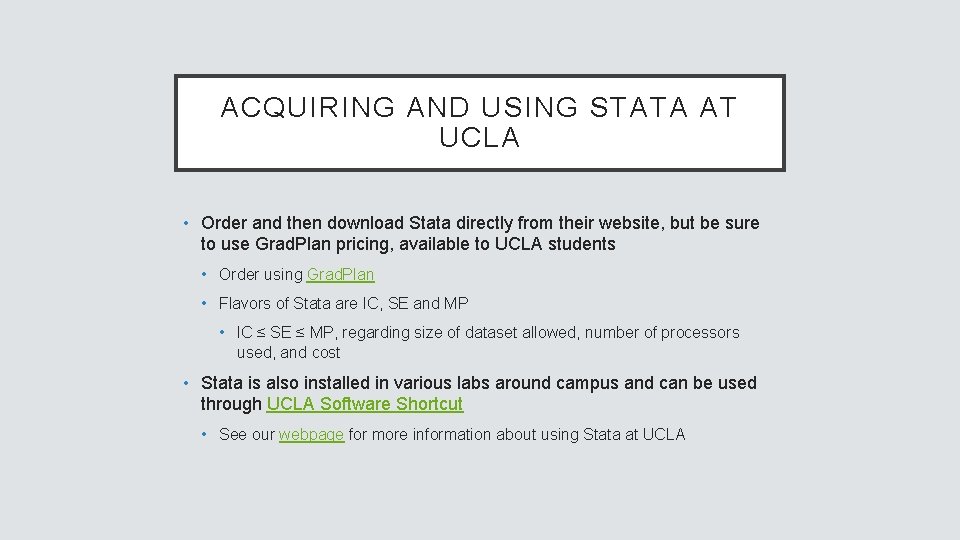
ACQUIRING AND USING STATA AT UCLA • Order and then download Stata directly from their website, but be sure to use Grad. Plan pricing, available to UCLA students • Order using Grad. Plan • Flavors of Stata are IC, SE and MP • IC ≤ SE ≤ MP, regarding size of dataset allowed, number of processors used, and cost • Stata is also installed in various labs around campus and can be used through UCLA Software Shortcut • See our webpage for more information about using Stata at UCLA

NAVIGATING STATA’S INTERFACE cd change working directory

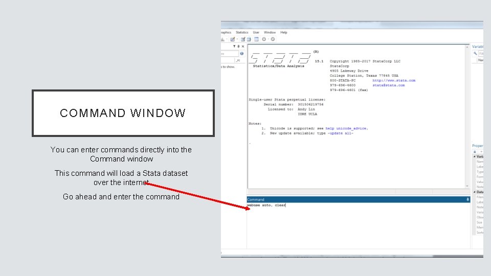
COMMAND WINDOW You can enter commands directly into the Command window This command will load a Stata dataset over the internet Go ahead and enter the command

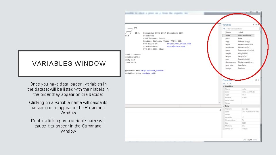
VARIABLES WINDOW Once you have data loaded, variables in the dataset will be listed with their labels in the order they appear on the dataset Clicking on a variable name will cause its description to appear in the Properties Window Double-clicking on a variable name will cause it to appear in the Command Window

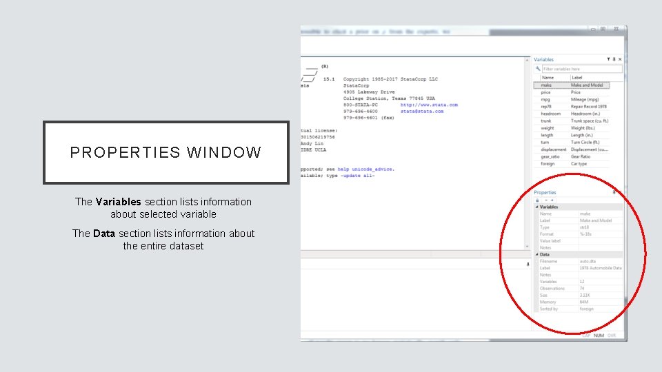
PROPERTIES WINDOW The Variables section lists information about selected variable The Data section lists information about the entire dataset

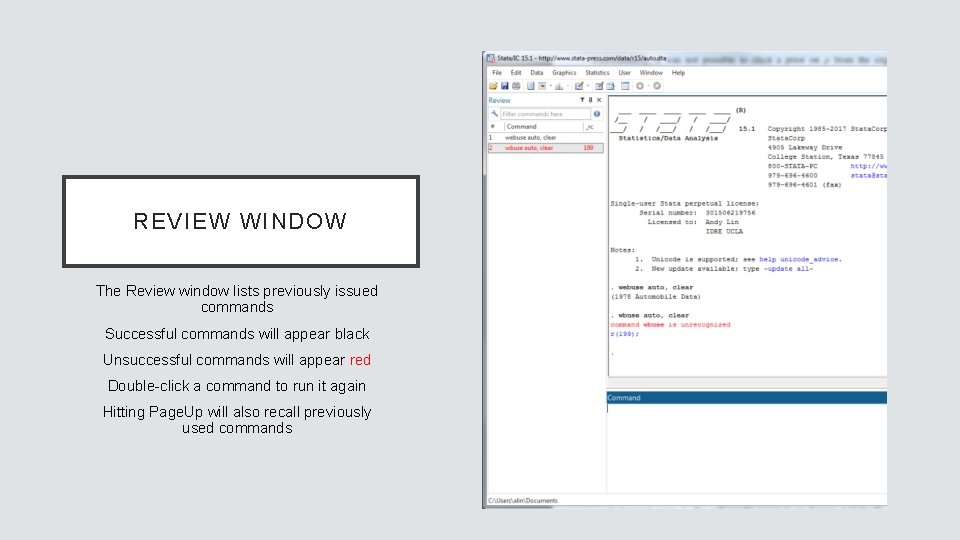
REVIEW WINDOW The Review window lists previously issued commands Successful commands will appear black Unsuccessful commands will appear red Double-click a command to run it again Hitting Page. Up will also recall previously used commands

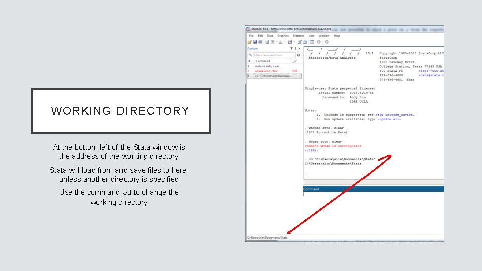
WORKING DIRECTORY At the bottom left of the Stata window is the address of the working directory Stata will load from and save files to here, unless another directory is specified Use the command cd to change the working directory

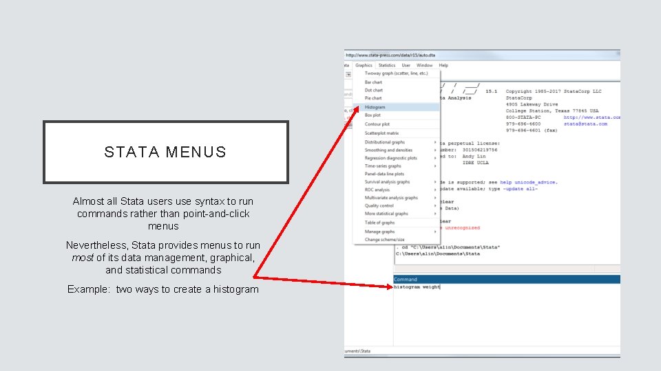
STATA MENUS Almost all Stata users use syntax to run commands rather than point-and-click menus Nevertheless, Stata provides menus to run most of its data management, graphical, and statistical commands Example: two ways to create a histogram

DO-FILES doedit open do-file editor

DO-FILES ARE SCRIPTS OF COMMANDS • Stata do-files are text files where users can store and run their commands for reuse, rather than retyping the commands into the Command window • Reproducibility • Easier debugging and changing commands • We recommend always using a do-file when using Stata • The file extension. do is used for do-files

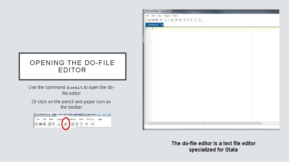
OPENING THE DO-FILE EDITOR Use the command doedit to open the dofile editor Or click on the pencil and paper icon on the toolbar The do-file editor is a text file editor specialized for Stata

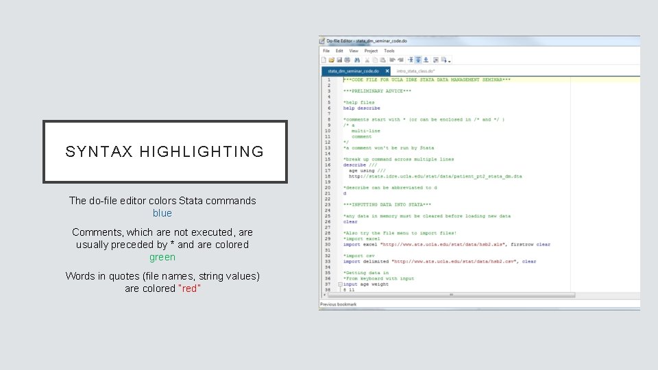
SYNTAX HIGHLIGHTING The do-file editor colors Stata commands blue Comments, which are not executed, are usually preceded by * and are colored green Words in quotes (file names, string values) are colored “red”

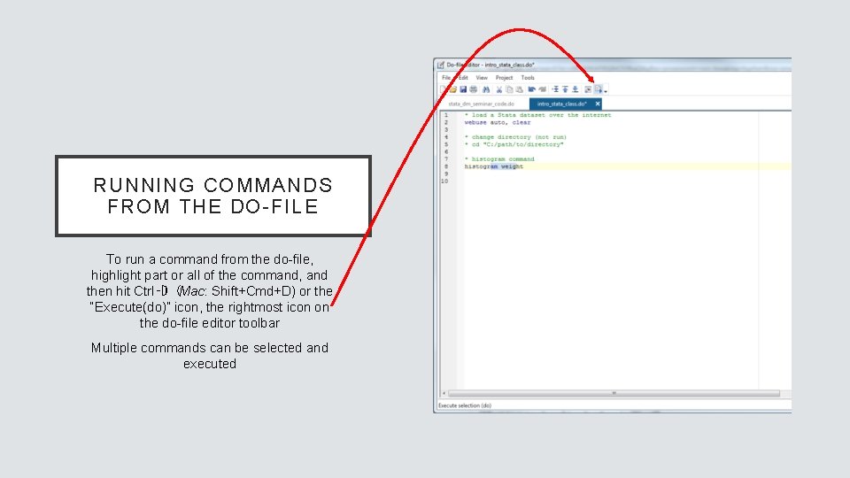
RUNNING COMMANDS FROM THE DO-FILE To run a command from the do-file, highlight part or all of the command, and then hit Ctrl‑D (Mac: Shift+Cmd+D) or the “Execute(do)” icon, the rightmost icon on the do-file editor toolbar Multiple commands can be selected and executed

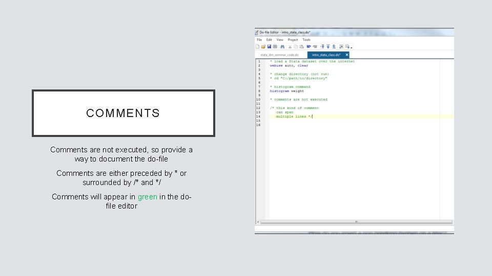
COMMENTS Comments are not executed, so provide a way to document the do-file Comments are either preceded by * or surrounded by /* and */ Comments will appear in green in the dofile editor

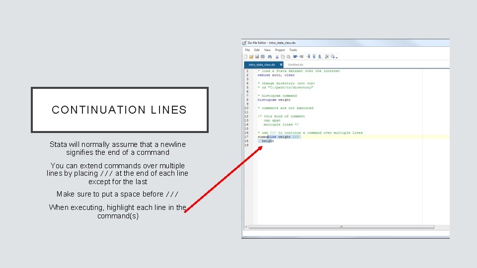
CONTINUATION LINES Stata will normally assume that a newline signifies the end of a command You can extend commands over multiple lines by placing /// at the end of each line except for the last Make sure to put a space before /// When executing, highlight each line in the command(s)

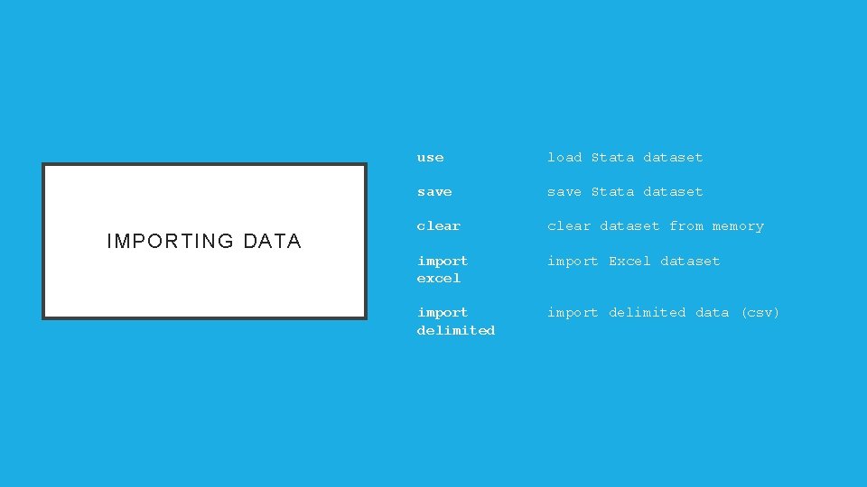
IMPORTING DATA use load Stata dataset save Stata dataset clear dataset from memory import excel import Excel dataset import delimited data (csv)

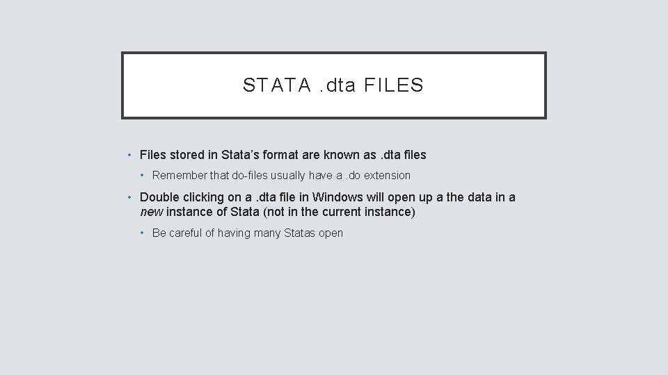
STATA. dta FILES • Files stored in Stata’s format are known as. dta files • Remember that do-files usually have a. do extension • Double clicking on a. dta file in Windows will open up a the data in a new instance of Stata (not in the current instance) • Be careful of having many Statas open

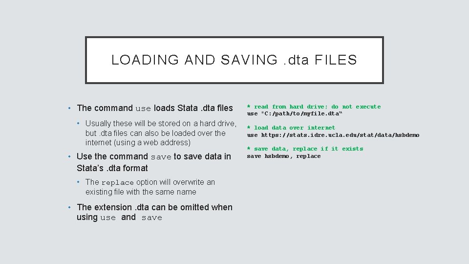
LOADING AND SAVING. dta FILES • The command use loads Stata. dta files • Usually these will be stored on a hard drive, but. dta files can also be loaded over the internet (using a web address) • Use the command save to save data in Stata’s. dta format • The replace option will overwrite an existing file with the same name • The extension. dta can be omitted when using use and save * read from hard drive; do not execute use "C: /path/to/myfile. dta“ * load data over internet use https: //stats. idre. ucla. edu/stat/data/hsbdemo * save data, replace if it exists save hsbdemo, replace

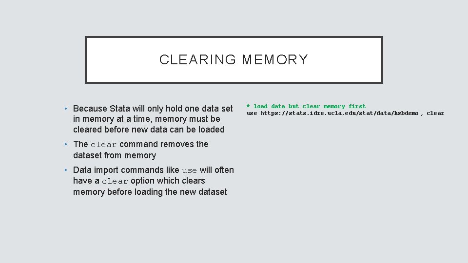
CLEARING MEMORY • Because Stata will only hold one data set in memory at a time, memory must be cleared before new data can be loaded • The clear command removes the dataset from memory • Data import commands like use will often have a clear option which clears memory before loading the new dataset * load data but clear memory first use https: //stats. idre. ucla. edu/stat/data/hsbdemo , clear

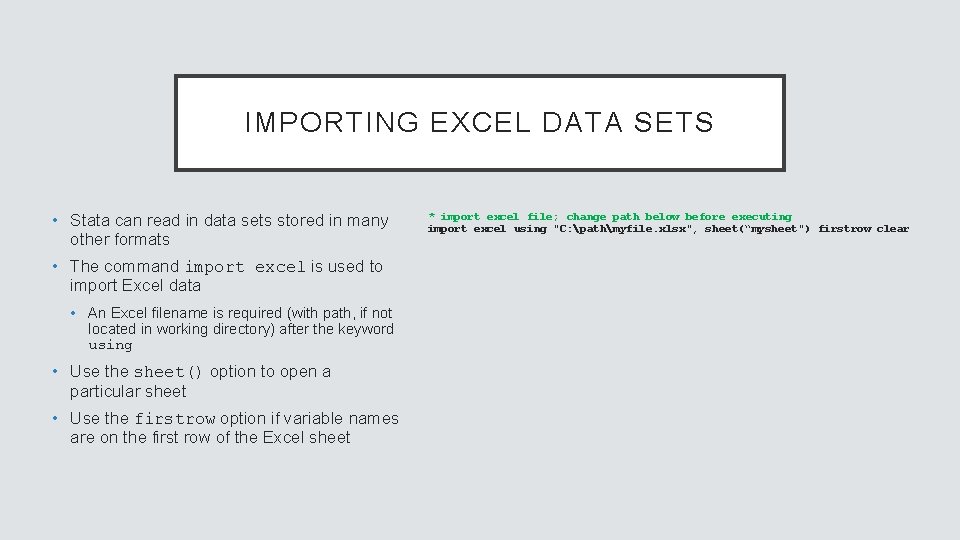
IMPORTING EXCEL DATA SETS • Stata can read in data sets stored in many other formats • The command import excel is used to import Excel data • An Excel filename is required (with path, if not located in working directory) after the keyword using • Use the sheet() option to open a particular sheet • Use the firstrow option if variable names are on the first row of the Excel sheet * import excel file; change path below before executing import excel using "C: pathmyfile. xlsx", sheet(“mysheet") firstrow clear

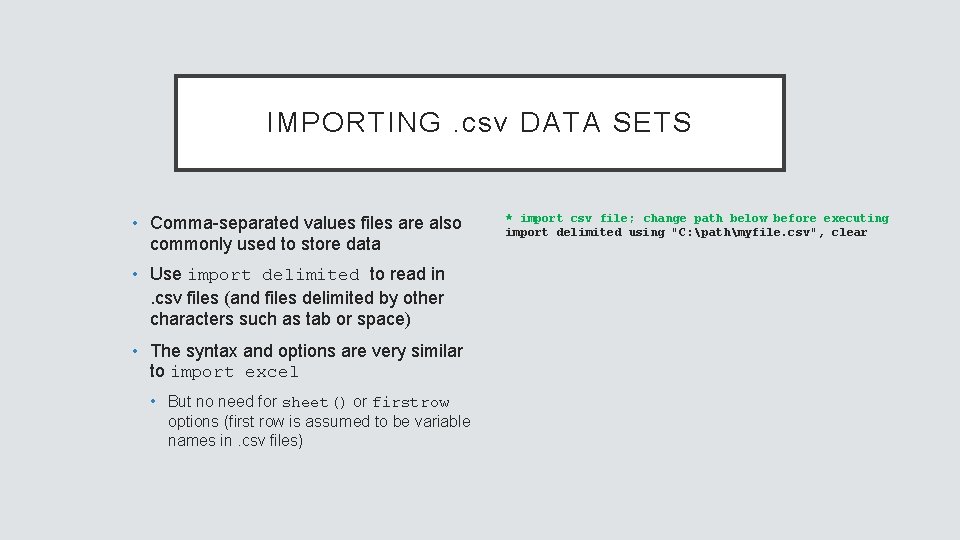
IMPORTING. csv DATA SETS • Comma-separated values files are also commonly used to store data • Use import delimited to read in . csv files (and files delimited by other characters such as tab or space) • The syntax and options are very similar to import excel • But no need for sheet() or firstrow options (first row is assumed to be variable names in. csv files) * import csv file; change path below before executing import delimited using "C: pathmyfile. csv", clear

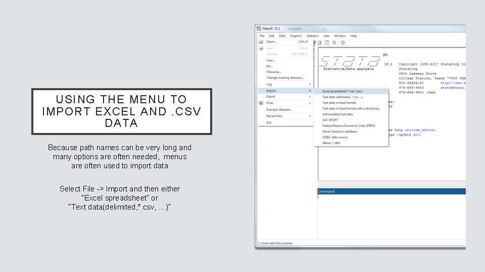
USING THE MENU TO IMPORT EXCEL AND. CSV DATA Because path names can be very long and many options are often needed, menus are often used to import data Select File -> Import and then either “Excel spreadsheet” or “Text data(delimited, *. csv, …)”

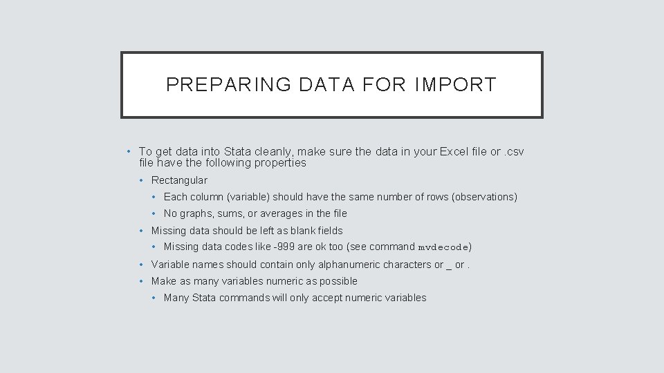
PREPARING DATA FOR IMPORT • To get data into Stata cleanly, make sure the data in your Excel file or. csv file have the following properties • Rectangular • Each column (variable) should have the same number of rows (observations) • No graphs, sums, or averages in the file • Missing data should be left as blank fields • Missing data codes like -999 are ok too (see command mvdecode) • Variable names should contain only alphanumeric characters or _ or. • Make as many variables numeric as possible • Many Stata commands will only accept numeric variables

HELP FILES AND STATA SYNTAX help command open help page for command

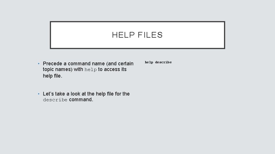
HELP FILES • Precede a command name (and certain topic names) with help to access its help file. • Let’s take a look at the help file for the describe command. help describe

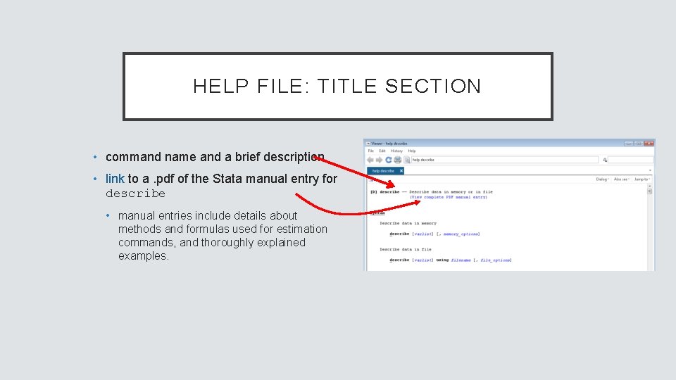
HELP FILE: TITLE SECTION • command name and a brief description • link to a. pdf of the Stata manual entry for describe • manual entries include details about methods and formulas used for estimation commands, and thoroughly explained examples.

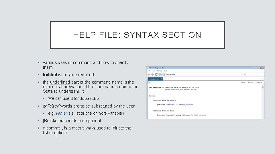
HELP FILE: SYNTAX SECTION • various uses of command how to specify them • bolded words are required • the underlined part of the command name is the minimal abbreviation of the command required for Stata to understand it • We can use d for describe • italicized words are to be substituted by the user • e. g. varlist is a list of one or more variables • [Bracketed] words are optional • a comma , is almost always used to initiate the list of options

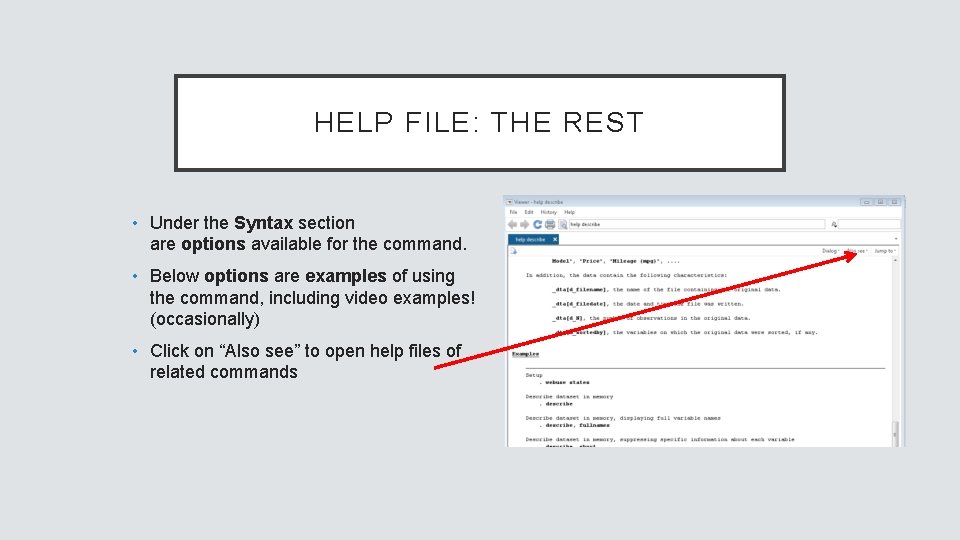
HELP FILE: THE REST • Under the Syntax section are options available for the command. • Below options are examples of using the command, including video examples! (occasionally) • Click on “Also see” to open help files of related commands

GETTING TO KNOW YOUR DATA

VIEWING DATA browse open spreadsheet of data list print data to Stata console

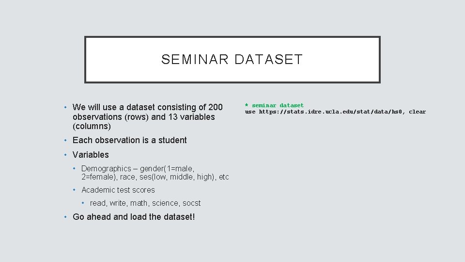
SEMINAR DATASET • We will use a dataset consisting of 200 observations (rows) and 13 variables (columns) • Each observation is a student • Variables • Demographics – gender(1=male, 2=female), race, ses(low, middle, high), etc • Academic test scores • read, write, math, science, socst • Go ahead and load the dataset! * seminar dataset use https: //stats. idre. ucla. edu/stat/data/hs 0, clear

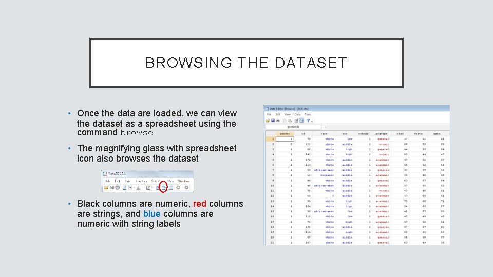
BROWSING THE DATASET • Once the data are loaded, we can view the dataset as a spreadsheet using the command browse • The magnifying glass with spreadsheet icon also browses the dataset • Black columns are numeric, red columns are strings, and blue columns are numeric with string labels

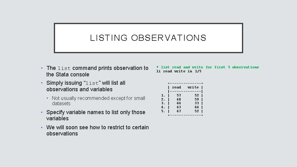
LISTING OBSERVATIONS • The list command prints observation to the Stata console * list read and write for first 5 observations li read write in 1/5 • Simply issuing “list” will list all observations and variables • Not usually recommended except for small datasets • Specify variable names to list only those variables • We will soon see how to restrict to certain observations 1. 2. 3. 4. 5. +-------+ | read write | |-------| | 57 52 | | 68 59 | | 44 33 | | 63 44 | | 47 52 | +-------+

SELECTING OBSERVATIONS in select by observation number if select by condition

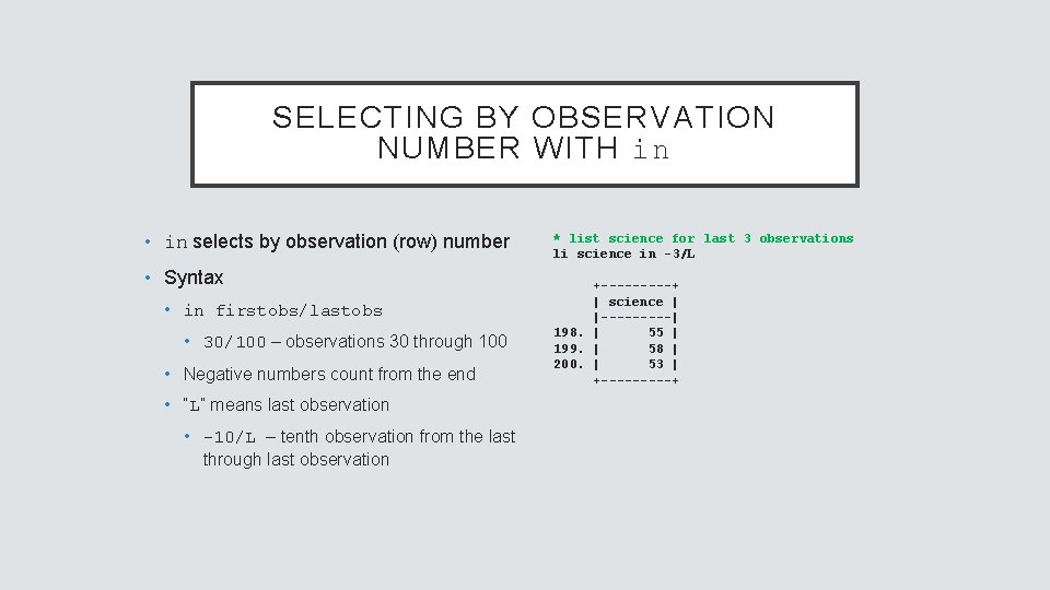
SELECTING BY OBSERVATION NUMBER WITH in • in selects by observation (row) number • Syntax • in firstobs/lastobs • 30/100 – observations 30 through 100 • Negative numbers count from the end • “L” means last observation • -10/L – tenth observation from the last through last observation * list science for last 3 observations li science in -3/L +-----+ | science | |-----| 198. | 55 | 199. | 58 | 200. | 53 | +-----+

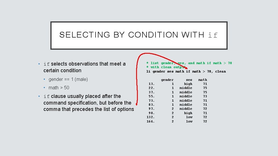
SELECTING BY CONDITION WITH if • if selects observations that meet a certain condition * list gender, ses, and math if math > 70 * with clean output li gender ses math if math > 70, clean • gender == 1 (male) • math > 50 • if clause usually placed after the command specification, but before the comma that precedes the list of options 13. 22. 37. 55. 73. 83. 97. 98. 132. 164. gender 1 1 1 2 2 ses high middle middle high low math 71 75 75 73 71 71 72 72

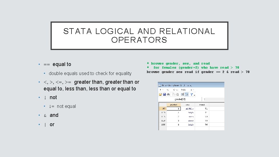
STATA LOGICAL AND RELATIONAL OPERATORS • == equal to • double equals used to check for equality • <, >, <=, >= greater than, greater than or equal to, less than or equal to • ! not • != not equal • & and • | or * browse gender, ses, and read * for females (gender=2) who have read > 70 browse gender ses read if gender == 2 & read > 70

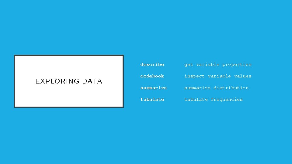
EXPLORING DATA describe get variable properties codebook inspect variable values summarize distribution tabulate frequencies

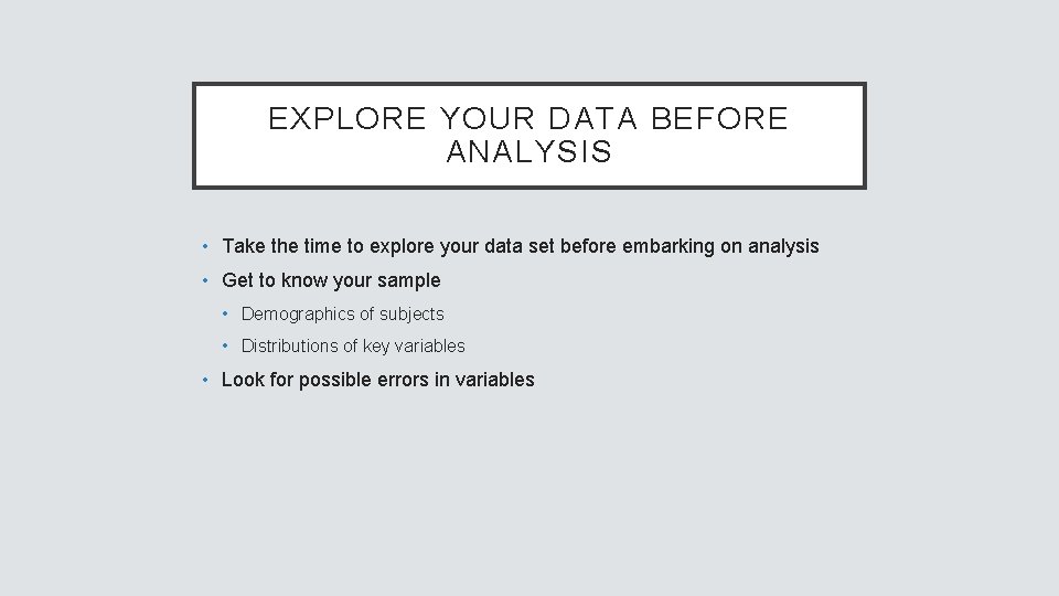
EXPLORE YOUR DATA BEFORE ANALYSIS • Take the time to explore your data set before embarking on analysis • Get to know your sample • Demographics of subjects • Distributions of key variables • Look for possible errors in variables

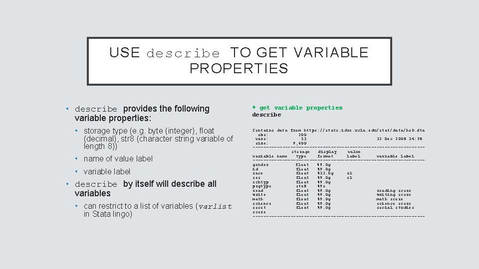
USE describe TO GET VARIABLE PROPERTIES • describe provides the following variable properties: • storage type (e. g. byte (integer), float (decimal), str 8 (character string variable of length 8)) • name of value label • variable label • describe by itself will describe all variables • can restrict to a list of variables (varlist in Stata lingo) * get variable properties describe Contains data from https: //stats. idre. ucla. edu/stat/data/hs 0. dta obs: 200 vars: 11 12 Dec 2008 14: 38 size: 9, 600 --------------------------------storage display value variable name type format label variable label --------------------------------gender float %9. 0 g id float %9. 0 g race float %12. 0 g rl ses float %9. 0 g sl schtyp float %9. 0 g prgtype str 8 %9 s read float %9. 0 g reading score write float %9. 0 g writing score math float %9. 0 g math score science float %9. 0 g science score socst float %9. 0 g social studies score --------------------------------

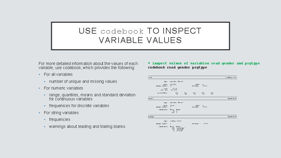
USE codebook TO INSPECT VARIABLE VALUES For more detailed information about the values of each variable, use codebook, which provides the following: • For all variables • number of unique and missing values • For numeric variables • range, quantiles, means and standard deviation for continuous variables • frequenices for discrete variables • For string variables • frequencies • warnings about leading and trailing blanks * inspect values of variables read gender and prgtype codebook read gender prgtype --------------------------------------------------reading score --------------------------------------------------type: range: unique values: numeric (float) [28, 76] 30 mean: std. dev: units: missing. : 1 0/200 52. 23 10. 2529 percentiles: 10% 39 25% 44 50% 50 75% 60 90% 67 --------------------------------------------------gender (unlabeled) --------------------------------------------------type: numeric (float) range: unique values: [1, 2] 2 tabulation: Freq. 91 109 units: missing. : 1 0/200 Value 1 2 --------------------------------------------------prgtype (unlabeled) --------------------------------------------------type: unique values: tabulation: string (str 8) 3 Freq. 105 45 50 missing "": Value "academic" "general" "vocati" 0/200

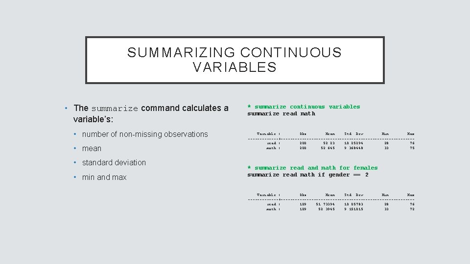
SUMMARIZING CONTINUOUS VARIABLES • The summarize command calculates a variable’s: • number of non-missing observations • mean • standard deviation • min and max * summarize continuous variables summarize read math Variable | Obs Mean Std. Dev. Min Max -------+----------------------------read | 200 52. 23 10. 25294 28 76 math | 200 52. 645 9. 368448 33 75 * summarize read and math for females summarize read math if gender == 2 Variable | Obs Mean Std. Dev. Min Max -------+----------------------------read | 109 51. 73394 10. 05783 28 76 math | 109 52. 3945 9. 151015 33 72

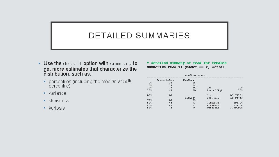
DETAILED SUMMARIES • Use the detail option with summary to get more estimates that characterize the distribution, such as: • percentiles (including the median at 50 th percentile) • variance • skewness • kurtosis * detailed summary of read for females summarize read if gender == 2, detail reading score ------------------------------Percentiles Smallest 1% 34 28 5% 36 34 10% 39 34 Obs 109 25% 44 35 Sum of Wgt. 109 50% 50 75% 90% 95% 99% 57 68 68 73 Largest 71 73 73 76 Mean Std. Dev. 51. 73394 10. 05783 Variance Skewness Kurtosis 101. 16. 3234174 2. 500028

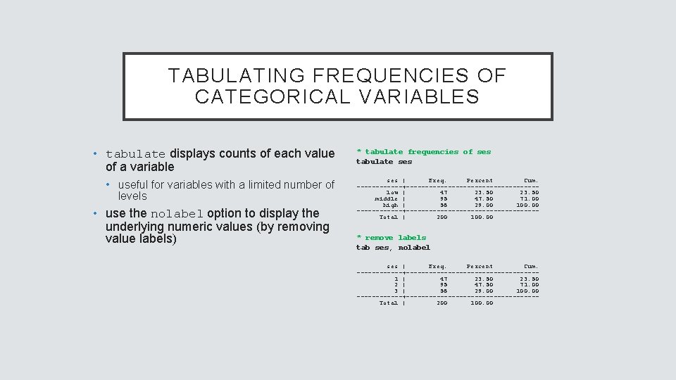
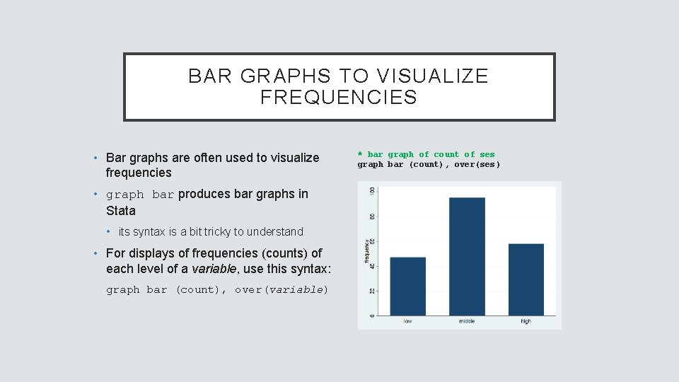
TABULATING FREQUENCIES OF CATEGORICAL VARIABLES • tabulate displays counts of each value of a variable • useful for variables with a limited number of levels • use the nolabel option to display the underlying numeric values (by removing value labels) * tabulate frequencies of ses tabulate ses | Freq. Percent Cum. ------+-----------------low | 47 23. 50 middle | 95 47. 50 71. 00 high | 58 29. 00 100. 00 ------+-----------------Total | 200 100. 00 * remove labels tab ses, nolabel ses | Freq. Percent Cum. ------+-----------------1 | 47 23. 50 2 | 95 47. 50 71. 00 3 | 58 29. 00 100. 00 ------+-----------------Total | 200 100. 00

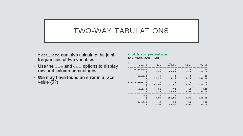
TWO-WAY TABULATIONS • tabulate can also calculate the joint frequencies of two variables • Use the row and col options to display row and column percentages • We may have found an error in a race value (5? ) * with row percentages tab race ses, row | ses race | low middle high | Total -------+-----------------+-----hispanic | 9 11 4 | 24 | 37. 50 45. 83 16. 67 | 100. 00 -------+-----------------+-----asian | 3 5 3 | 11 | 27. 27 45. 45 27. 27 | 100. 00 -------+-----------------+-----african-amer | 11 6 3 | 20 | 55. 00 30. 00 15. 00 | 100. 00 -------+-----------------+-----white | 24 71 48 | 143 | 16. 78 49. 65 33. 57 | 100. 00 -------+-----------------+-----5 | 0 2 0 | 2 | 0. 00 100. 00 | 100. 00 -------+-----------------+-----Total | 47 95 58 | 200 | 23. 50 47. 50 29. 00 | 100. 00

DATA VISUALIZATION histogram graph boxplot scatter plot graph bar plots

DATA VISUALIZATION • Data visualization is the representation of data in visual formats such as graphs • Graphs help us to gain information about the distributions of variables and relationships among variables quickly through visual inspection • Graphs can be used to explore your data, to familiarize yourself with distributions and associations in your data • Graphs can also be used to present the results of statistical analysis

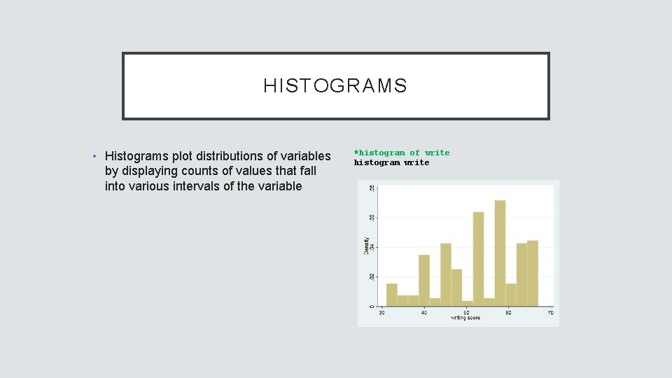
HISTOGRAMS • Histograms plot distributions of variables by displaying counts of values that fall into various intervals of the variable *histogram of write histogram write

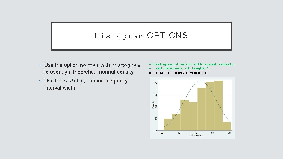
histogram OPTIONS • Use the option normal with histogram to overlay a theoretical normal density • Use the width() option to specify interval width * histogram of write with normal density * and intervals of length 5 hist write, normal width(5)

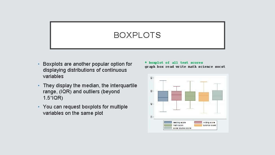
BOXPLOTS • Boxplots are another popular option for displaying distributions of continuous variables • They display the median, the interquartile range, (IQR) and outliers (beyond 1. 5*IQR) • You can request boxplots for multiple variables on the same plot * boxplot of all test scores graph box read write math science socst

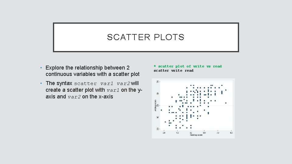
SCATTER PLOTS • Explore the relationship between 2 continuous variables with a scatter plot • The syntax scatter var 1 var 2 will create a scatter plot with var 1 on the yaxis and var 2 on the x-axis * scatter plot of write vs read scatter write read

BAR GRAPHS TO VISUALIZE FREQUENCIES • Bar graphs are often used to visualize frequencies • graph bar produces bar graphs in Stata • its syntax is a bit tricky to understand • For displays of frequencies (counts) of each level of a variable, use this syntax: graph bar (count), over(variable) * bar graph of count of ses graph bar (count), over(ses )

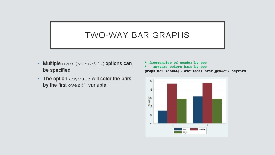
TWO-WAY BAR GRAPHS • Multiple over(variable)options can be specified • The option asyvars will color the bars by the first over() variable * frequencies of gender by ses * asyvars colors bars by ses graph bar (count), over(ses) over(gender) asyvars

TWO-WAY, LAYERED GRAPHICS • The Stata graphing command twoway produces layered graphics, where multiple plots can be overlayed on the same graph • Each plot should involve a y-variable and an x-variable that appear on the y-axis and x-axis, respectively • Syntax (generally): twoway (plottype 1 yvar xvar) (plottype 2 yvar xvar)… • plottype is one of several types of plots available to twoway, and yvar and xvar are the variables to appear on the y-axis and x-axis • See help twoway for a list of the many plottypes available

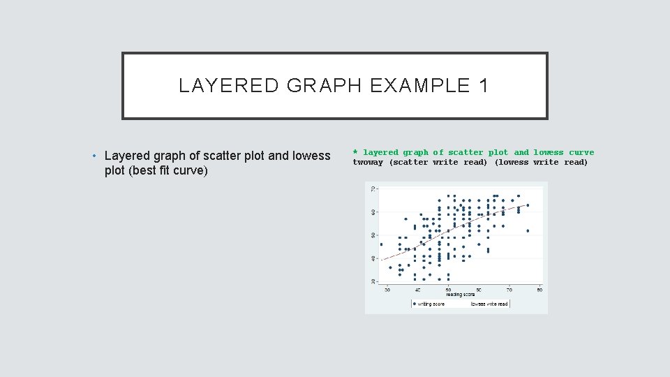
LAYERED GRAPH EXAMPLE 1 • Layered graph of scatter plot and lowess plot (best fit curve) * layered graph of scatter plot and lowess curve twoway (scatter write read) (lowess write read)

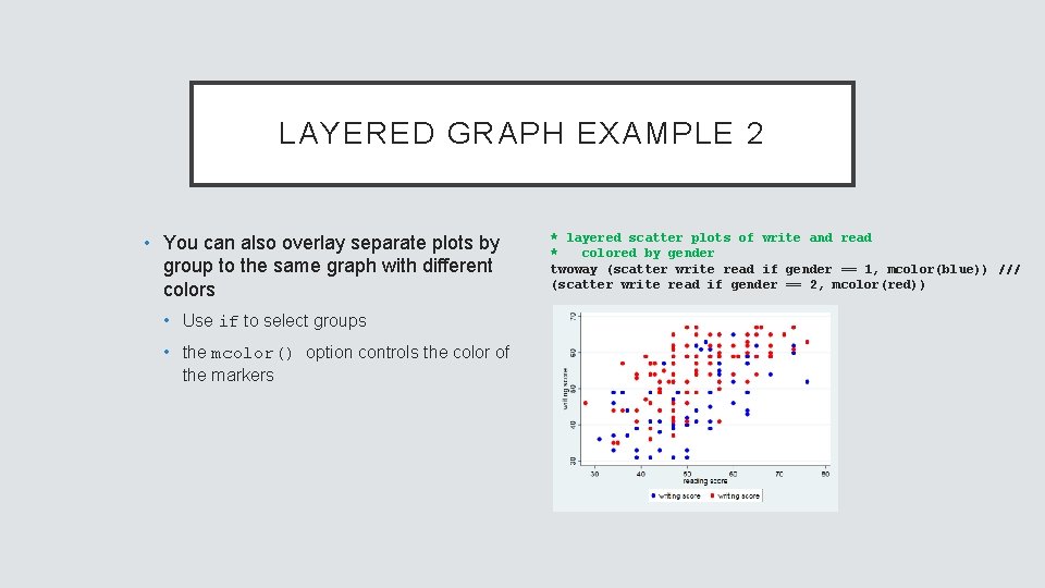
LAYERED GRAPH EXAMPLE 2 • You can also overlay separate plots by group to the same graph with different colors • Use if to select groups • the mcolor() option controls the color of the markers * layered scatter plots of write and read * colored by gender twoway (scatter write read if gender == 1, mcolor(blue)) /// (scatter write read if gender == 2, mcolor(red))

DATA MANAGEMENT

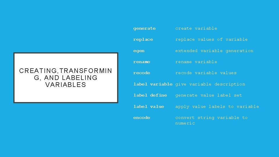
CREATING, TRANSFORMIN G, AND LABELING VARIABLES generate create variable replace values of variable egen extended variable generation rename variable recode variable values label variable give variable description label define generate value label set label value apply value labels to variable encode convert string variable to numeric

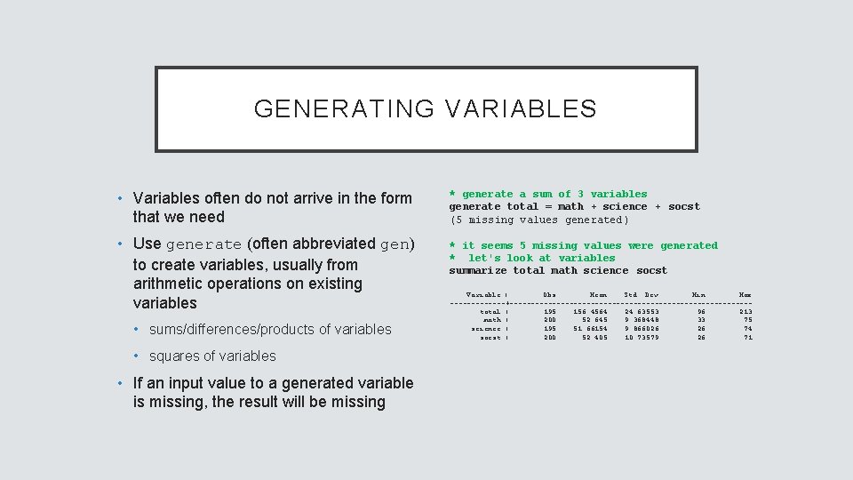
GENERATING VARIABLES • Variables often do not arrive in the form that we need * generate a sum of 3 variables generate total = math + science + socst (5 missing values generated ) • Use generate (often abbreviated gen) to create variables, usually from arithmetic operations on existing variables * it seems 5 missing values were generated * let's look at variables summarize total math science socst • sums/differences/products of variables • squares of variables • If an input value to a generated variable is missing, the result will be missing Variable | Obs Mean Std. Dev. Min Max -------+----------------------------total | 195 156. 4564 24. 63553 96 213 math | 200 52. 645 9. 368448 33 75 science | 195 51. 66154 9. 866026 26 74 socst | 200 52. 405 10. 73579 26 71

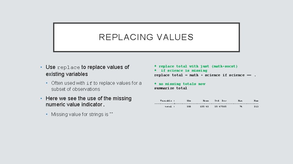
REPLACING VALUES • Use replace to replace values of existing variables • Often used with if to replace values for a subset of observations • Here we see the use of the missing numeric value indicator. • Missing value for strings is “” * replace total with just (math+socst) * if science is missing replace total = math + science if science ==. * no missing totals now summarize total Variable | Obs Mean Std. Dev. Min Max -------+----------------------------total | 200 155. 42 25. 47565 74 213

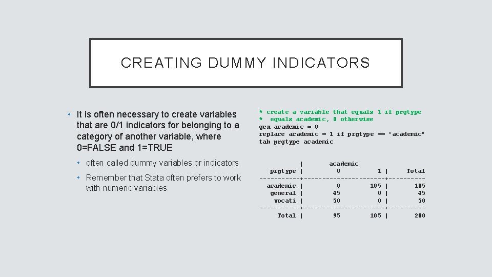
CREATING DUMMY INDICATORS • It is often necessary to create variables that are 0/1 indicators for belonging to a category of another variable, where 0=FALSE and 1=TRUE • often called dummy variables or indicators • Remember that Stata often prefers to work with numeric variables * create a variable that equals 1 if prgtype * equals academic, 0 otherwise gen academic = 0 replace academic = 1 if prgtype == "academic" tab prgtype academic | academic prgtype | 0 1 | Total ------+-----------+-----academic | 0 105 | 105 general | 45 0 | 45 vocati | 50 0 | 50 ------+-----------+-----Total | 95 105 | 200

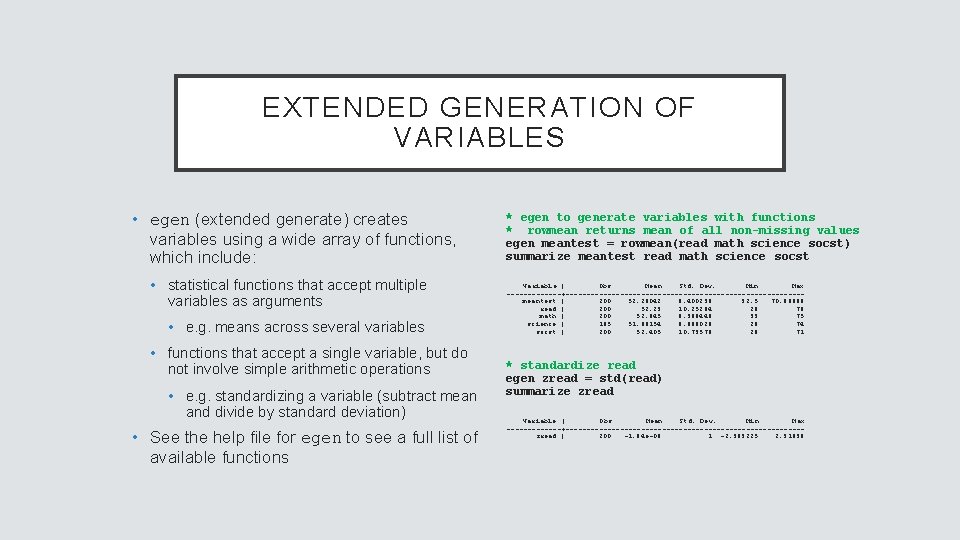
EXTENDED GENERATION OF VARIABLES • egen (extended generate) creates variables using a wide array of functions, which include: • statistical functions that accept multiple variables as arguments • e. g. means across several variables • functions that accept a single variable, but do not involve simple arithmetic operations • e. g. standardizing a variable (subtract mean and divide by standard deviation) • See the help file for egen to see a full list of available functions * egen to generate variables with functions * rowmean returns mean of all non-missing values egen meantest = rowmean(read math science socst) summarize meantest read math science socst Variable | Obs Mean Std. Dev. Min Max -------+----------------------------meantest | 200 52. 28042 8. 400239 32. 5 70. 66666 read | 200 52. 23 10. 25294 28 76 math | 200 52. 645 9. 368448 33 75 science | 195 51. 66154 9. 866026 26 74 socst | 200 52. 405 10. 73579 26 71 * standardize read egen zread = std(read) summarize zread Variable | Obs Mean Std. Dev. Min Max -------+----------------------------zread | 200 -1. 84 e-09 1 -2. 363225 2. 31836

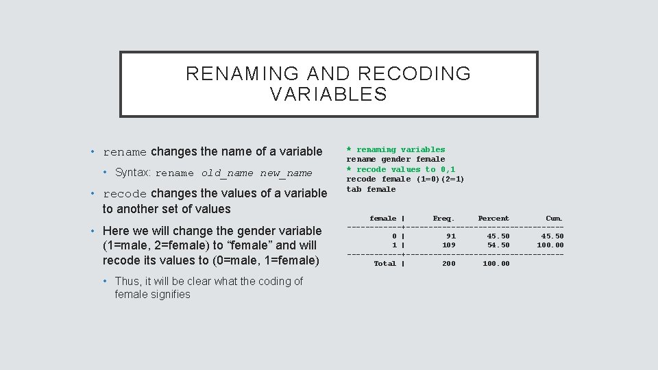
RENAMING AND RECODING VARIABLES • rename changes the name of a variable • Syntax: rename old_name new_name • recode changes the values of a variable to another set of values • Here we will change the gender variable (1=male, 2=female) to “female” and will recode its values to (0=male, 1=female) • Thus, it will be clear what the coding of female signifies * renaming variables rename gender female * recode values to 0, 1 recode female (1=0)(2=1) tab female | Freq. Percent Cum. ------+-----------------0 | 91 45. 50 1 | 109 54. 50 100. 00 ------+-----------------Total | 200 100. 00

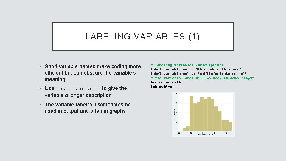
LABELING VARIABLES (1) • Short variable names make coding more efficient but can obscure the variable’s meaning • Use label variable to give the variable a longer description • The variable label will sometimes be used in output and often in graphs * labeling variables (description) label variable math "9 th grade math score” label variable schtyp "public/private school" * the variable label will be used in some output histogram math tab schtyp

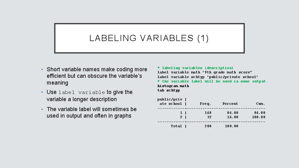
LABELING VARIABLES (1) • Short variable names make coding more efficient but can obscure the variable’s meaning • Use label variable to give the variable a longer description • The variable label will sometimes be used in output and often in graphs * labeling variables (description) label variable math "9 th grade math score” label variable schtyp "public/private school" * the variable label will be used in some output histogram math tab schtyp public/priv | ate school | Freq. Percent Cum. ------+-----------------1 | 168 84. 00 2 | 32 16. 00 100. 00 ------+-----------------Total | 200 100. 00

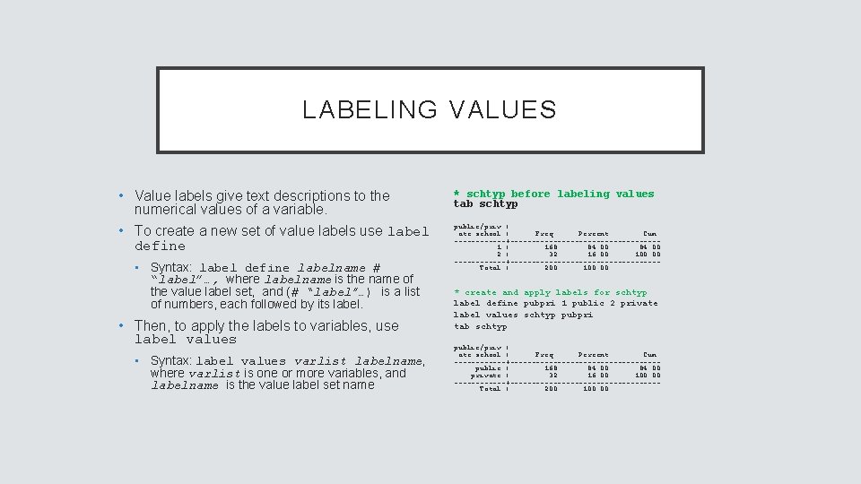
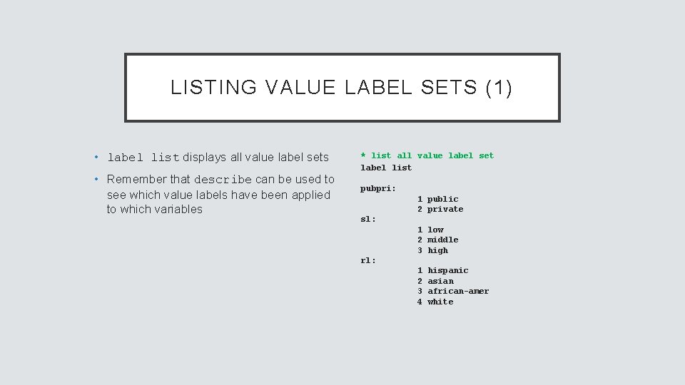
LABELING VALUES • Value labels give text descriptions to the numerical values of a variable. • To create a new set of value labels use label define • Syntax: label define labelname # “label”…, where labelname is the name of the value label set, and (# “label”…) is a list of numbers, each followed by its label. • Then, to apply the labels to variables, use label values • Syntax: label values varlist labelname, where varlist is one or more variables, and labelname is the value label set name * schtyp before labeling values tab schtyp public/priv | ate school | Freq. Percent Cum. ------+-----------------1 | 168 84. 00 2 | 32 16. 00 100. 00 ------+-----------------Total | 200 100. 00 * create and apply labels for schtyp label define pubpri 1 public 2 private label values schtyp pubpri tab schtyp public/priv | ate school | Freq. Percent Cum. ------+-----------------public | 168 84. 00 private | 32 16. 00 100. 00 ------+-----------------Total | 200 100. 00

LISTING VALUE LABEL SETS (1) • label list displays all value label sets • Remember that describe can be used to see which value labels have been applied to which variables * list all value label set label list pubpri: 1 public 2 private sl: 1 low 2 middle 3 high rl: 1 2 3 4 hispanic asian african-amer white

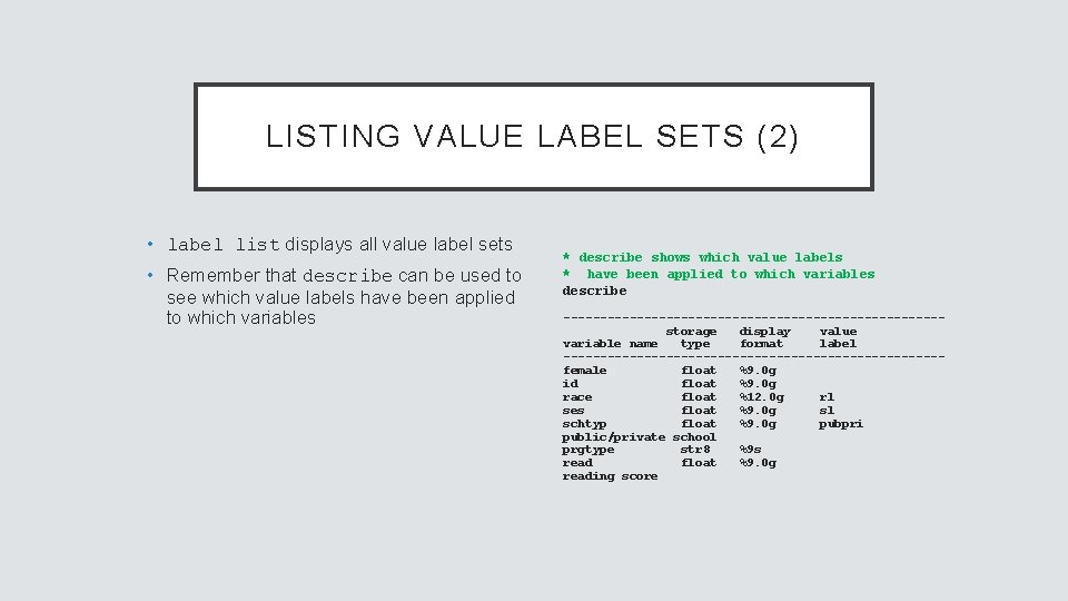
LISTING VALUE LABEL SETS (2) • label list displays all value label sets • Remember that describe can be used to see which value labels have been applied to which variables * describe shows which value labels * have been applied to which variables describe --------------------------storage display value variable name type format label --------------------------female float %9. 0 g id float %9. 0 g race float %12. 0 g rl ses float %9. 0 g sl schtyp float %9. 0 g pubpri public/private school prgtype str 8 %9 s read float %9. 0 g reading score

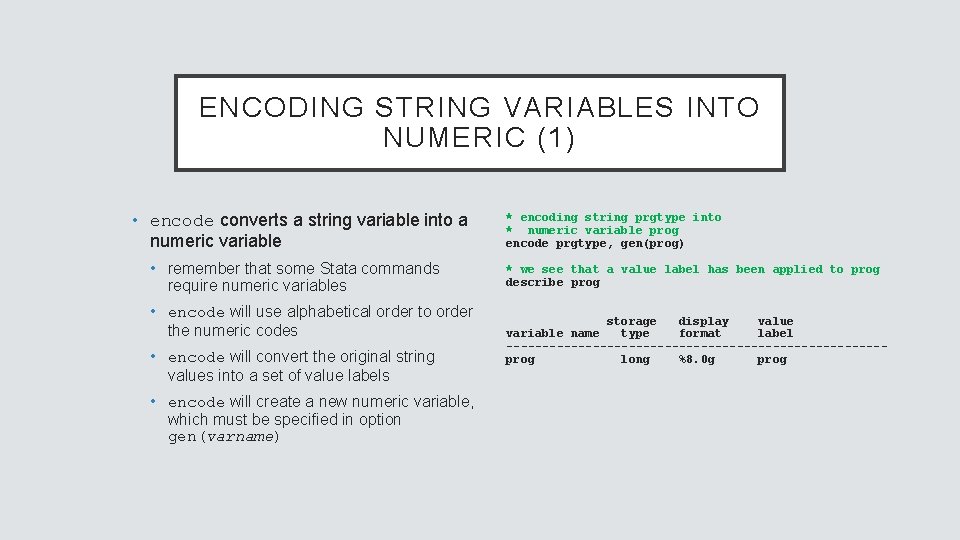
ENCODING STRING VARIABLES INTO NUMERIC (1) • encode converts a string variable into a numeric variable • remember that some Stata commands require numeric variables • encode will use alphabetical order to order the numeric codes • encode will convert the original string values into a set of value labels • encode will create a new numeric variable, which must be specified in option gen(varname) * encoding string prgtype into * numeric variable prog encode prgtype, gen(prog) * we see that a value label has been applied to prog describe prog storage display value variable name type format label --------------------------prog long %8. 0 g prog

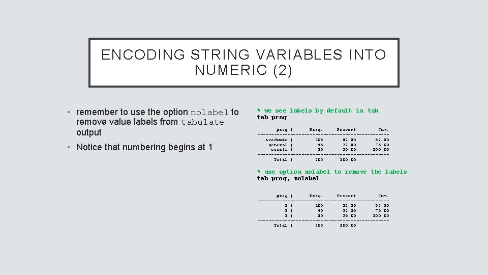
ENCODING STRING VARIABLES INTO NUMERIC (2) • remember to use the option nolabel to remove value labels from tabulate output • Notice that numbering begins at 1 * we see labels by default in tab prog | Freq. Percent Cum. ------+-----------------academic | 105 52. 50 general | 45 22. 50 75. 00 vocati | 50 25. 00 100. 00 ------+-----------------Total | 200 100. 00 * use option nolabel to remove the labels tab prog, nolabel prog | Freq. Percent Cum. ------+-----------------1 | 105 52. 50 2 | 45 22. 50 75. 00 3 | 50 25. 00 100. 00 ------+-----------------Total | 200 100. 00

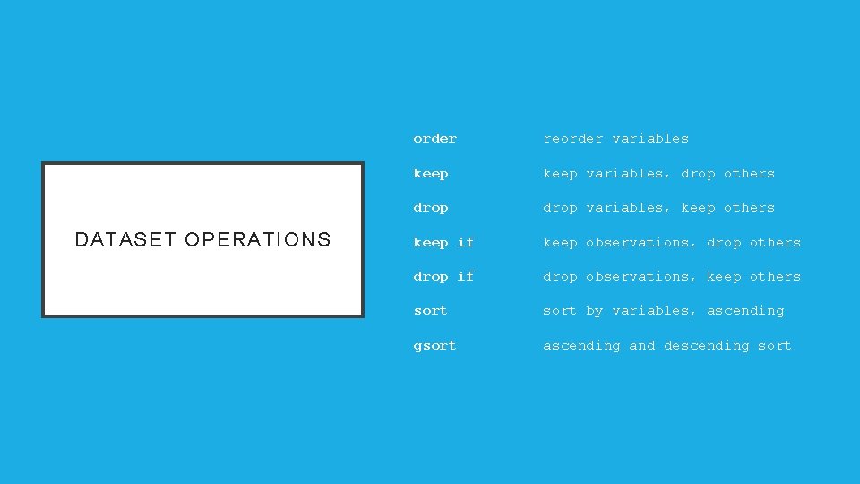
DATASET OPERATIONS order reorder variables keep variables, drop others drop variables, keep others keep if keep observations, drop others drop if drop observations, keep others sort by variables, ascending gsort ascending and descending sort

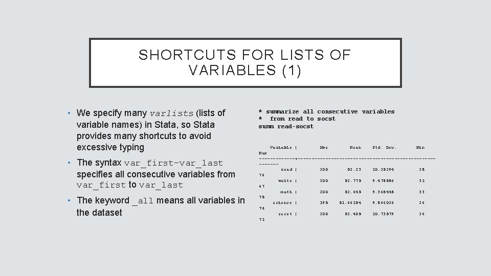
SHORTCUTS FOR LISTS OF VARIABLES (1) • We specify many varlists (lists of variable names) in Stata, so Stata provides many shortcuts to avoid excessive typing • The syntax var_first-var_last specifies all consecutive variables from var_first to var_last • The keyword _all means all variables in the dataset * summarize all consecutive variables * from read to socst summ read-socst Variable | Obs Mean Std. Dev. Min Max -------+----------------------------read | 200 52. 23 10. 25294 28 76 write | 200 52. 775 9. 478586 31 67 math | 200 52. 645 9. 368448 33 75 science | 195 51. 66154 9. 866026 26 74 socst | 200 52. 405 10. 73579 26 71

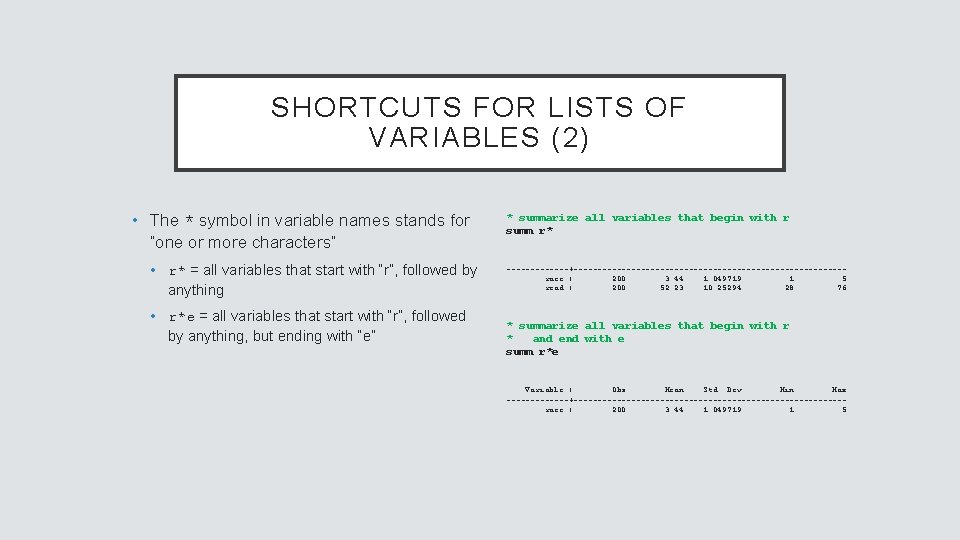
SHORTCUTS FOR LISTS OF VARIABLES (2) • The * symbol in variable names stands for “one or more characters” • r* = all variables that start with “r”, followed by anything • r*e = all variables that start with “r”, followed by anything, but ending with “e” * summarize all variables that begin with r summ r* -------+----------------------------race | 200 3. 44 1. 049719 1 5 read | 200 52. 23 10. 25294 28 76 * summarize all variables that begin with r * and end with e summ r*e Variable | Obs Mean Std. Dev. Min Max -------+----------------------------race | 200 3. 44 1. 049719 1 5

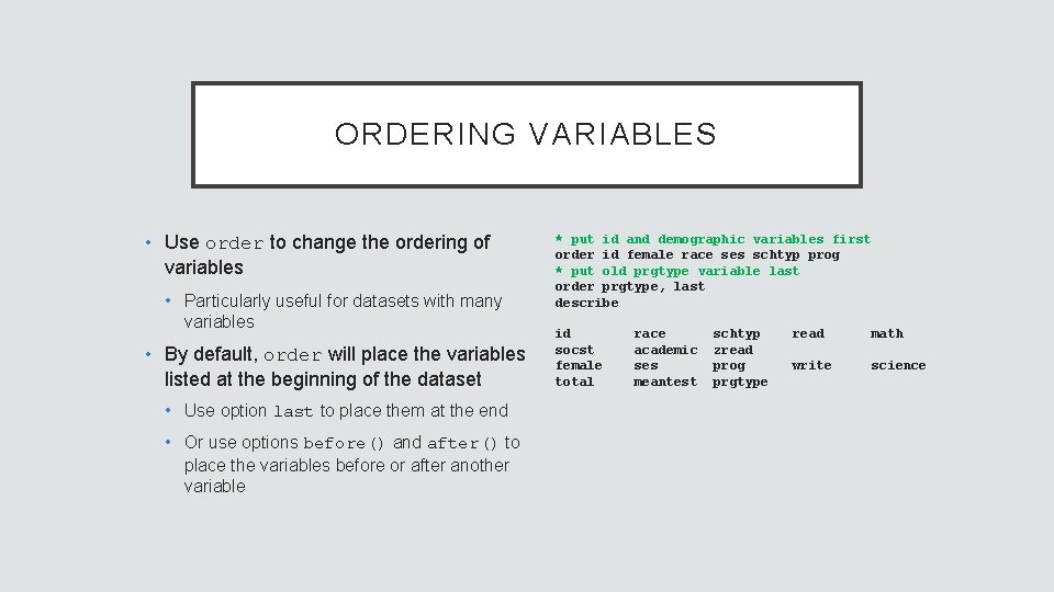
ORDERING VARIABLES • Use order to change the ordering of variables • Particularly useful for datasets with many variables • By default, order will place the variables listed at the beginning of the dataset • Use option last to place them at the end • Or use options before() and after() to place the variables before or after another variable * put id and demographic variables first order id female race ses schtyp prog * put old prgtype variable last order prgtype, last describe id socst female total race academic ses meantest schtyp zread prog prgtype read math write science

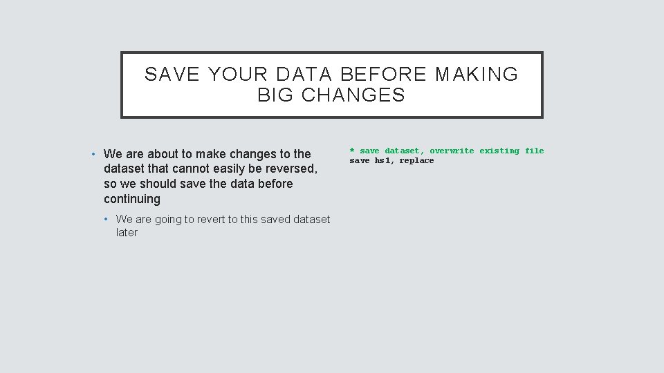
SAVE YOUR DATA BEFORE MAKING BIG CHANGES • We are about to make changes to the dataset that cannot easily be reversed, so we should save the data before continuing • We are going to revert to this saved dataset later * save dataset, overwrite existing file save hs 1, replace

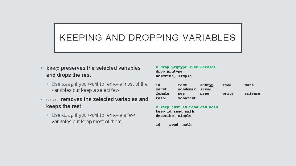
KEEPING AND DROPPING VARIABLES • keep preserves the selected variables and drops the rest • Use keep if you want to remove most of the variables but keep a select few • drop removes the selected variables and keeps the rest • Use drop if you want to remove a few variables but keep most of them * drop prgtype from dataset drop prgtype describe, simple id socst female total race academic ses meantest schtyp zread prog * keep just id read and math keep id read math describe, simple id read math write science

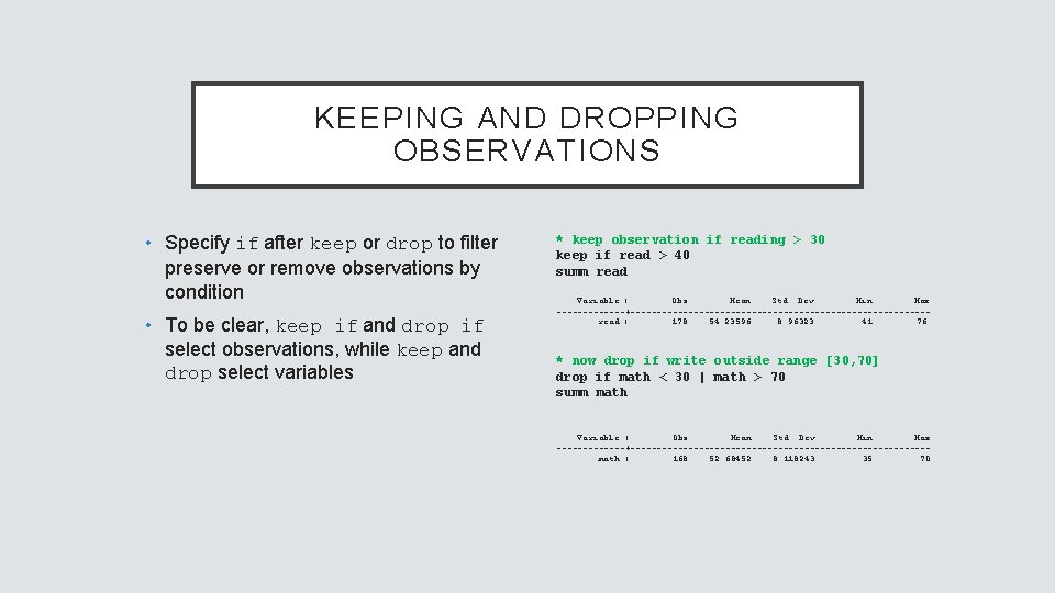
KEEPING AND DROPPING OBSERVATIONS • Specify if after keep or drop to filter preserve or remove observations by condition • To be clear, keep if and drop if select observations, while keep and drop select variables * keep observation if reading > 30 keep if read > 40 summ read Variable | Obs Mean Std. Dev. Min Max -------+----------------------------read | 178 54. 23596 8. 96323 41 76 * now drop if write outside range [30, 70] drop if math < 30 | math > 70 summ math Variable | Obs Mean Std. Dev. Min Max -------+----------------------------math | 168 52. 68452 8. 118243 35 70

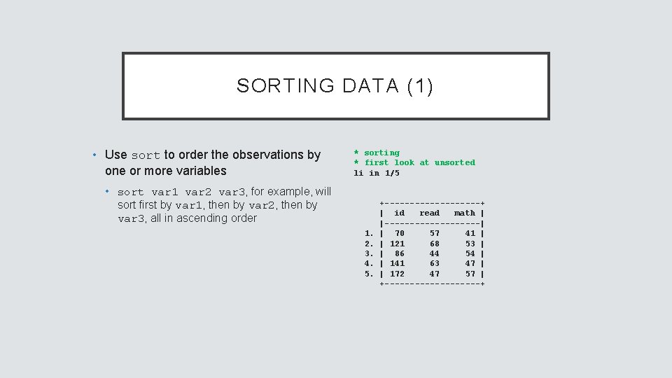
SORTING DATA (1) • Use sort to order the observations by one or more variables * sorting * first look at unsorted li in 1/5 • sort var 1 var 2 var 3, for example, will sort first by var 1, then by var 2, then by var 3, all in ascending order 1. 2. 3. 4. 5. +----------+ | id read math | |----------| | 70 57 41 | | 121 68 53 | | 86 44 54 | | 141 63 47 | | 172 47 57 | +----------+

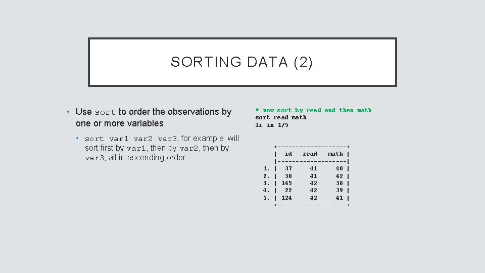
SORTING DATA (2) • Use sort to order the observations by one or more variables * now sort by read and then math sort read math li in 1/5 • sort var 1 var 2 var 3, for example, will sort first by var 1, then by var 2, then by var 3, all in ascending order 1. 2. 3. 4. 5. +----------+ | id read math | |----------| | 37 41 40 | | 30 41 42 | | 145 42 38 | | 22 42 39 | | 124 42 41 | +----------+

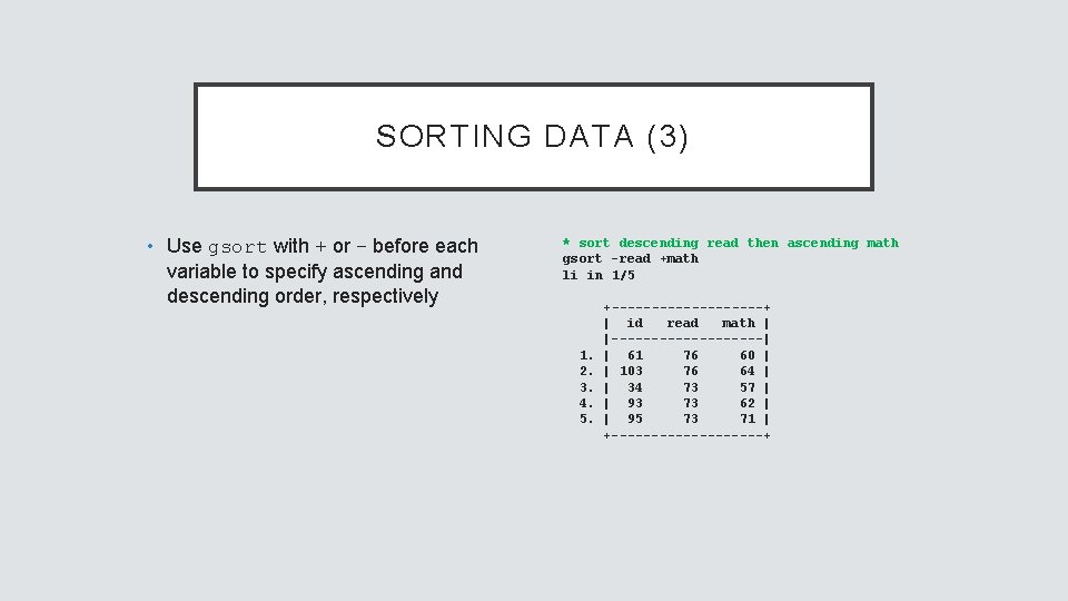
SORTING DATA (3) • Use gsort with + or – before each variable to specify ascending and descending order, respectively * sort descending read then ascending math gsort -read +math li in 1/5 1. 2. 3. 4. 5. +----------+ | id read math | |----------| | 61 76 60 | | 103 76 64 | | 34 73 57 | | 93 73 62 | | 95 73 71 | +----------+

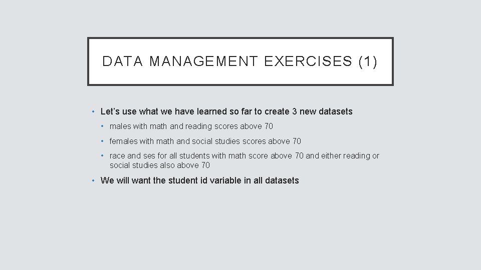
DATA MANAGEMENT EXERCISES (1) • Let’s use what we have learned so far to create 3 new datasets • males with math and reading scores above 70 • females with math and social studies scores above 70 • race and ses for all students with math score above 70 and either reading or social studies also above 70 • We will want the student id variable in all datasets

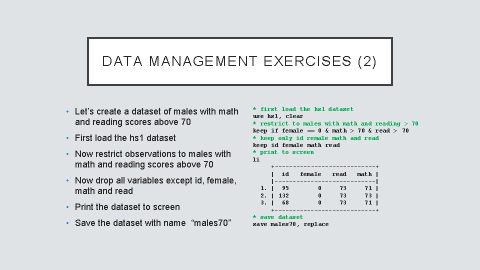
DATA MANAGEMENT EXERCISES (2) • Let’s create a dataset of males with math and reading scores above 70 • First load the hs 1 dataset • Now restrict observations to males with math and reading scores above 70 • Now drop all variables except id, female, math and read • Print the dataset to screen • Save the dataset with name “males 70” * first load the hs 1 dataset use hs 1, clear * restrict to males with math and reading > 70 keep if female == 0 & math > 70 & read > 70 * keep only id remale math and read keep id female math read * print to screen li +--------------+ | id female read math | |--------------| 1. | 95 0 73 71 | 2. | 132 0 73 73 | 3. | 68 0 73 71 | +--------------+ * save dataset save males 70, replace

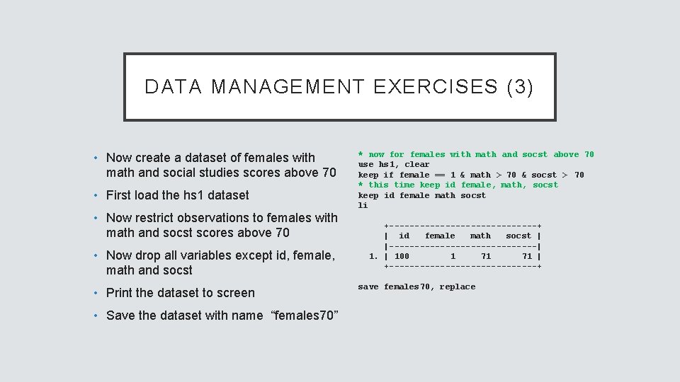
DATA MANAGEMENT EXERCISES (3) • Now create a dataset of females with math and social studies scores above 70 • First load the hs 1 dataset • Now restrict observations to females with math and socst scores above 70 • Now drop all variables except id, female, math and socst • Print the dataset to screen • Save the dataset with name “females 70” * now for females with math and socst above 70 use hs 1, clear keep if female == 1 & math > 70 & socst > 70 * this time keep id female, math, socst keep id female math socst li +---------------+ | id female math socst | |---------------| 1. | 100 1 71 71 | +---------------+ save females 70, replace

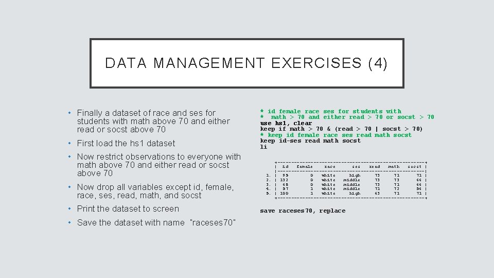
DATA MANAGEMENT EXERCISES (4) • Finally a dataset of race and ses for students with math above 70 and either read or socst above 70 • First load the hs 1 dataset • Now restrict observations to everyone with math above 70 and either read or socst above 70 • Now drop all variables except id, female, race, ses, read, math, and socst • Print the dataset to screen • Save the dataset with name “raceses 70” * id female race ses for students with * math > 70 and either read > 70 or socst > 70 use hs 1, clear keep if math > 70 & (read > 70 | socst > 70) * keep id female race ses read math socst keep id-ses read math socst li 1. 2. 3. 4. 5. +---------------------------+ | id female race ses read math socst | |---------------------------| | 95 0 white high 73 71 71 | | 132 0 white middle 73 73 66 | | 68 0 white middle 73 71 66 | | 57 1 white middle 71 72 56 | | 100 1 white high 63 71 71 | +---------------------------+ save raceses 70, replace

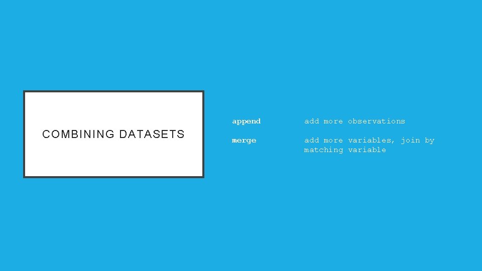
COMBINING DATASETS append add more observations merge add more variables, join by matching variable

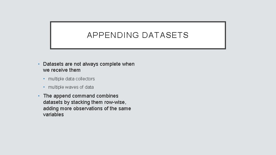
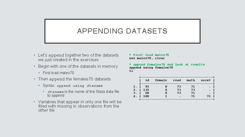
APPENDING DATASETS • Datasets are not always complete when we receive them • multiple data collectors • multiple waves of data • The append command combines datasets by stacking them row-wise, adding more observations of the same variables

APPENDING DATASETS • Let’s append together two of the datasets we just created in the exercises * first load males 70 use males 70, clear • Begin with one of the datasets in memory * append females 70 and look at results append using females 70 li • First load males 70 • Then append the females 70 datasets • Syntax: append using dtaname • dtaname is the name of the Stata data file to append • Variables that appear in only one file will be filled with missing in observations from the other file 1. 2. 3. 4. +------------------+ | id female read math socst | |------------------| | 95 0 73 71. | | 132 0 73 73. | | 68 0 73 71. | | 100 1. 71 71 | +------------------+

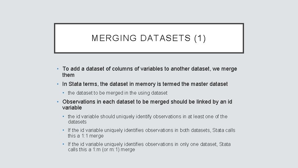
MERGING DATASETS (1) • To add a dataset of columns of variables to another dataset, we merge them • In Stata terms, the dataset in memory is termed the master dataset • the dataset to be merged in the using dataset • Observations in each dataset to be merged should be linked by an id variable • the id variable should uniquely identify observations in at least one of the datasets • If the id variable uniquely identifies observations in both datasets, Stata calls this a 1: 1 merge • If the id variable uniquely identifies observations in only one dataset, Stata calls this a 1: m (or m: 1) merge

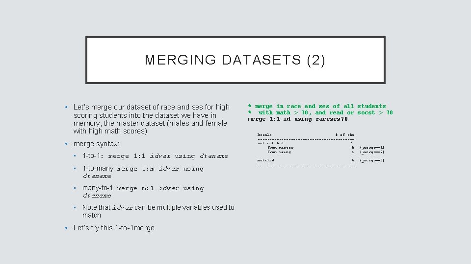
MERGING DATASETS (2) • Let’s merge our dataset of race and ses for high scoring students into the dataset we have in memory, the master dataset (males and female with high math scores) • merge syntax: • 1 -to-1: merge 1: 1 idvar using dtaname • 1 -to-many: merge 1: m idvar using dtaname • many-to-1: merge m: 1 idvar using dtaname • Note that idvar can be multiple variables used to match • Let’s try this 1 -to-1 merge * merge in race and ses of all students * with math > 70, and read or socst > 70 merge 1: 1 id using raceses 70 Result # of obs. --------------------not matched 1 from master 0 (_merge==1) from using 1 (_merge==2) matched 4 --------------------- (_merge==3)

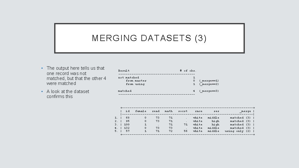
MERGING DATASETS (3) • The output here tells us that one record was not matched, but that the other 4 were matched Result # of obs. --------------------not matched 1 from master 0 (_merge==1) from using 1 (_merge==2) • A look at the dataset confirms this matched 4 --------------------- 1. 2. 3. 4. 5. (_merge==3) +-----------------------------------+ | id female read math socst race ses _merge | |-----------------------------------| | 68 0 73 71. white middle matched (3) | | 95 0 73 71. white high matched (3) | | 100 1. 71 71 white high matched (3) | | 132 0 73 73. white middle matched (3) | | 57 1 71 72 56 white middle using only (2) | +-----------------------------------+

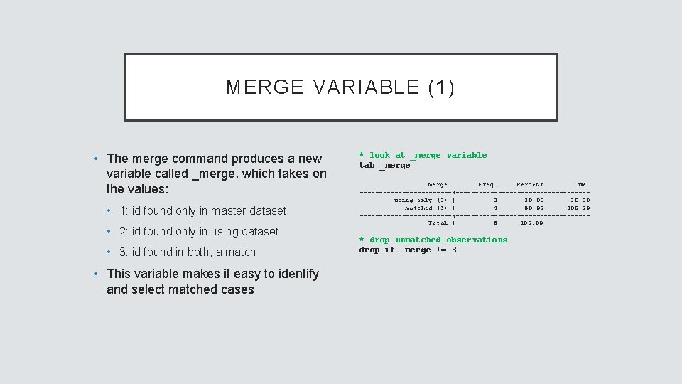
MERGE VARIABLE (1) • The merge command produces a new variable called _merge, which takes on the values: • 1: id found only in master dataset • 2: id found only in using dataset • 3: id found in both, a match • This variable makes it easy to identify and select matched cases * look at _merge variable tab _merge | Freq. Percent Cum. ------------+-----------------using only (2) | 1 20. 00 matched (3) | 4 80. 00 100. 00 ------------+-----------------Total | 5 100. 00 * drop unmatched observations drop if _merge != 3

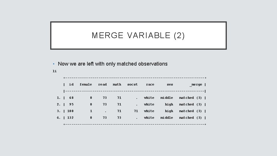
MERGE VARIABLE (2) • Now we are left with only matched observations li +----------------------------------+ | id female read math socst race ses _merge | |----------------------------------| 1. | 68 0 73 71 . white middle matched (3) | 2. | 95 0 73 71 . white high matched (3) | 3. | 100 1 . 71 71 white high matched (3) | 4. | 132 0 73 73 . white middle matched (3) | +----------------------------------+

BY-GROUP PROCESSING by varlist: execute command for each grouping of varlist

PROCESSING BY GROUP • We often want to perform data processing and statistical methods by group • Estimate means of a variable across groups • Rank along a variable within groups • Graph by group • We can precede many Stata commands with by varlist: to execute the command separately for each combination of levels of variables in varlist • Stata will want the data sorted by the varlist before executing a command by varlist • Stata provides the shortcut syntax bysort varlist: , which will sort first then execute by varlist

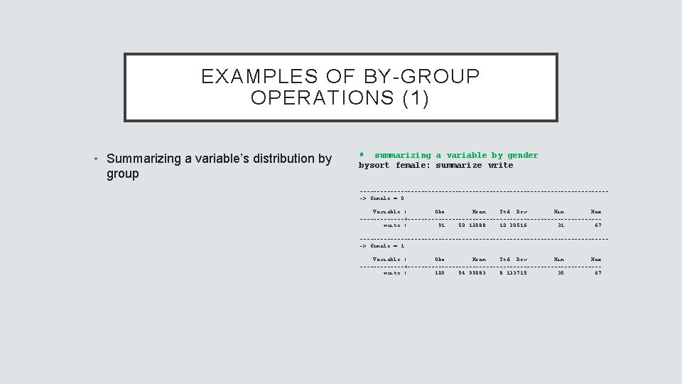
EXAMPLES OF BY-GROUP OPERATIONS (1) • Summarizing a variable’s distribution by group * summarizing a variable by gender bysort female: summarize write -------------------------------------> female = 0 Variable | Obs Mean Std. Dev. Min Max -------+----------------------------write | 91 50. 12088 10. 30516 31 67 -------------------------------------> female = 1 Variable | Obs Mean Std. Dev. Min Max -------+----------------------------write | 109 54. 99083 8. 133715 35 67

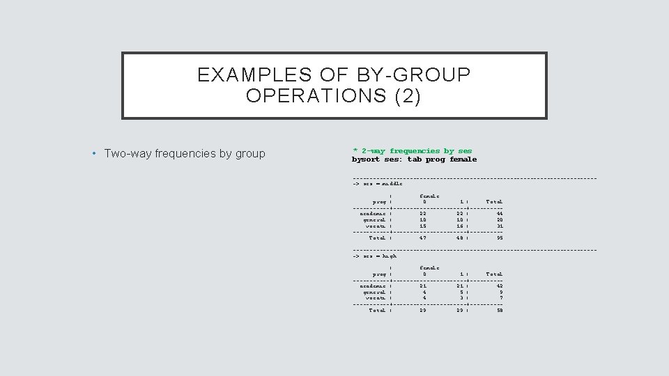
EXAMPLES OF BY-GROUP OPERATIONS (2) • Two-way frequencies by group * 2 -way frequencies by ses bysort ses: tab prog female -------------------------------------> ses = middle | female prog | 0 1 | Total ------+-----------+-----academic | 22 22 | 44 general | 10 10 | 20 vocati | 15 16 | 31 ------+-----------+-----Total | 47 48 | 95 -------------------------------------> ses = high | female prog | 0 1 | Total ------+-----------+-----academic | 21 21 | 42 general | 4 5 | 9 vocati | 4 3 | 7 ------+-----------+-----Total | 29 29 | 58

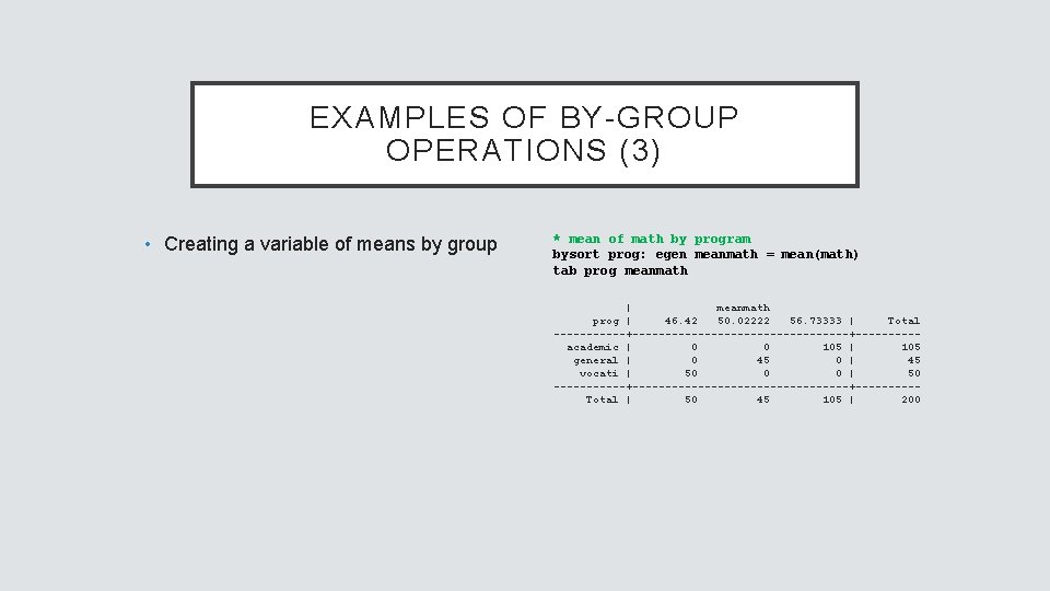
EXAMPLES OF BY-GROUP OPERATIONS (3) • Creating a variable of means by group * mean of math by program bysort prog: egen meanmath = mean(math) tab prog meanmath | meanmath prog | 46. 42 50. 02222 56. 73333 | Total ------+-----------------+-----academic | 0 0 105 | 105 general | 0 45 0 | 45 vocati | 50 0 0 | 50 ------+-----------------+-----Total | 50 45 105 | 200

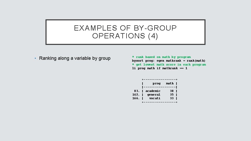
EXAMPLES OF BY-GROUP OPERATIONS (4) • Ranking along a variable by group * rank based bysort prog: * get lowest li prog math on math by program egen mathrank = rank(math) math score in each program if mathrank == 1 +---------+ | prog math | |---------| 83. | academic 38 | 142. | general 35 | 166. | vocati 33 | +---------+

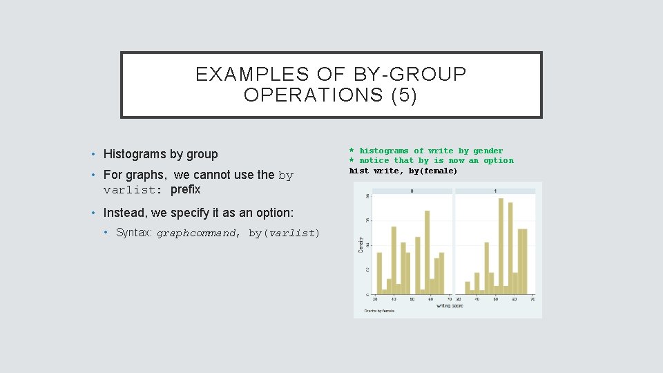
EXAMPLES OF BY-GROUP OPERATIONS (5) • Histograms by group • For graphs, we cannot use the by varlist: prefix • Instead, we specify it as an option: • Syntax: graphcommand, by(varlist) * histograms of write by gender * notice that by is now an option hist write, by(female)

BASIC STATISTICAL ANALYSIS

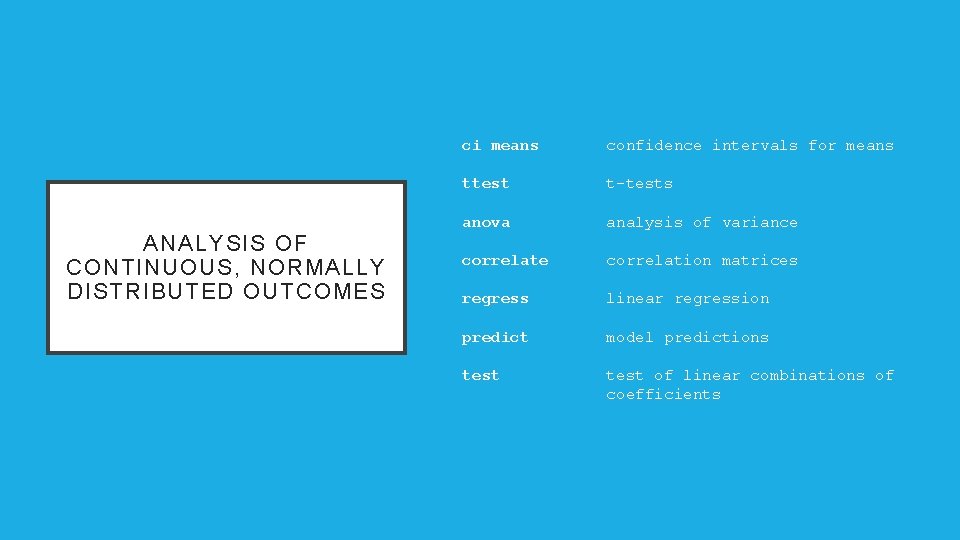
ANALYSIS OF CONTINUOUS, NORMALLY DISTRIBUTED OUTCOMES ci means confidence intervals for means ttest t-tests anova analysis of variance correlation matrices regress linear regression predict model predictions test of linear combinations of coefficients

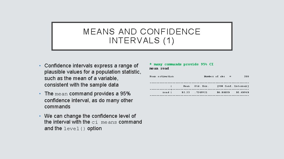
MEANS AND CONFIDENCE INTERVALS (1) • Confidence intervals express a range of plausible values for a population statistic, such as the mean of a variable, consistent with the sample data • The mean command provides a 95% confidence interval, as do many other commands • We can change the confidence level of the interval with the ci means command the level() option * many commands provide 95% CI mean read Mean estimation Number of obs = 200 -------------------------------| Mean Std. Err. [95% Conf. Interval] -------+------------------------read | 52. 23. 7249921 50. 80035 53. 65965 -------------------------------

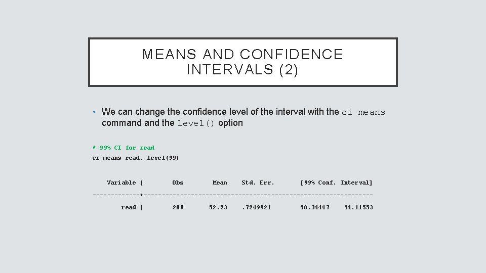
MEANS AND CONFIDENCE INTERVALS (2) • We can change the confidence level of the interval with the ci means command the level() option * 99% CI for read ci means read, level(99) Variable | Obs Mean Std. Err. [99% Conf. Interval] -------+-------------------------------read | 200 52. 23 . 7249921 50. 34447 54. 11553

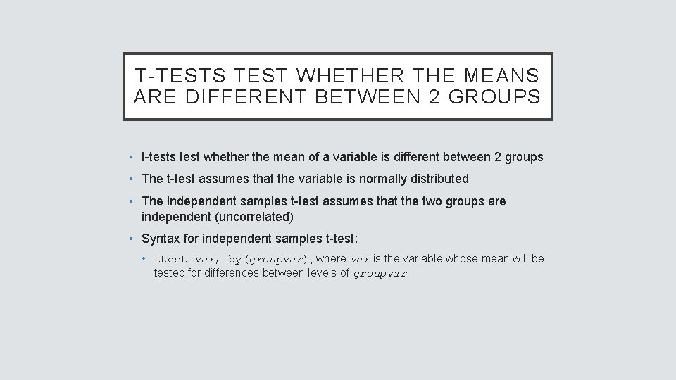
T-TESTS TEST WHETHER THE MEANS ARE DIFFERENT BETWEEN 2 GROUPS • t-tests test whether the mean of a variable is different between 2 groups • The t-test assumes that the variable is normally distributed • The independent samples t-test assumes that the two groups are independent (uncorrelated) • Syntax for independent samples t-test: • ttest var, by(groupvar), where var is the variable whose mean will be tested for differences between levels of groupvar

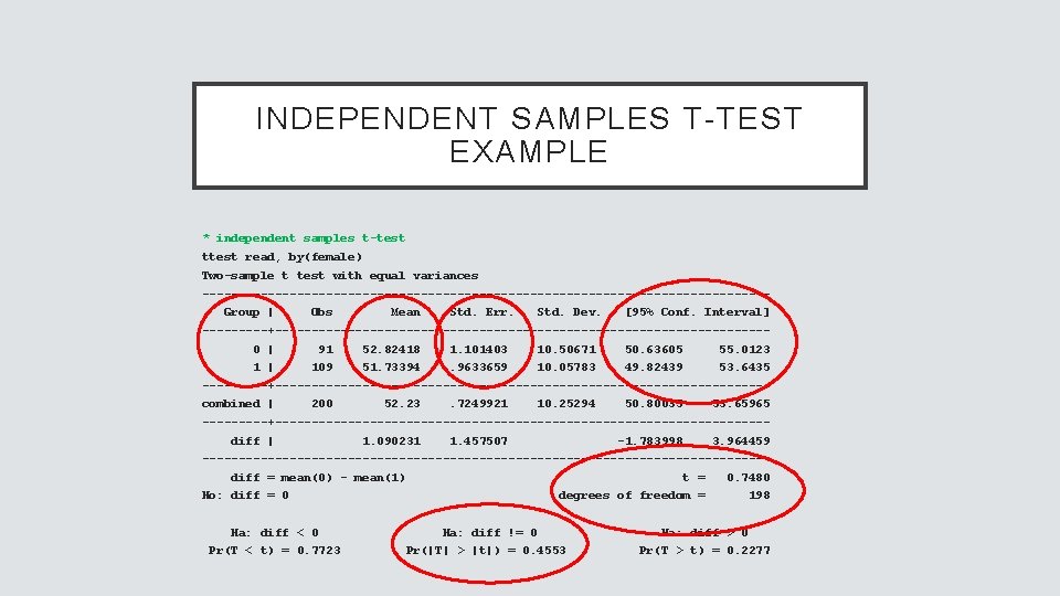
INDEPENDENT SAMPLES T-TEST EXAMPLE * independent samples t-test ttest read, by(female) Two-sample t test with equal variances ---------------------------------------Group | Obs Mean Std. Err. Std. Dev. [95% Conf. Interval] -----+----------------------------------0 | 91 52. 82418 1. 101403 10. 50671 50. 63605 55. 0123 1 | 109 51. 73394 . 9633659 10. 05783 49. 82439 53. 6435 -----+----------------------------------combined | 200 52. 23 . 7249921 10. 25294 50. 80035 53. 65965 -----+----------------------------------diff | 1. 090231 1. 457507 -1. 783998 3. 964459 ---------------------------------------diff = mean(0) - mean(1) Ho: diff = 0 t = 0. 7480 degrees of freedom = 198 Ha: diff < 0 Ha: diff != 0 Ha: diff > 0 Pr(T < t) = 0. 7723 Pr(|T| > |t|) = 0. 4553 Pr(T > t) = 0. 2277

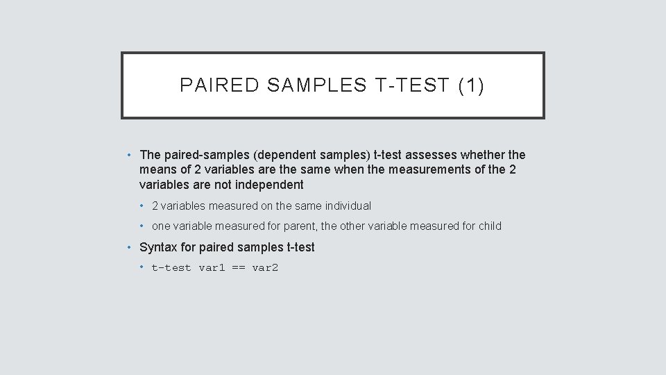
PAIRED SAMPLES T-TEST (1) • The paired-samples (dependent samples) t-test assesses whether the means of 2 variables are the same when the measurements of the 2 variables are not independent • 2 variables measured on the same individual • one variable measured for parent, the other variable measured for child • Syntax for paired samples t-test • t-test var 1 == var 2

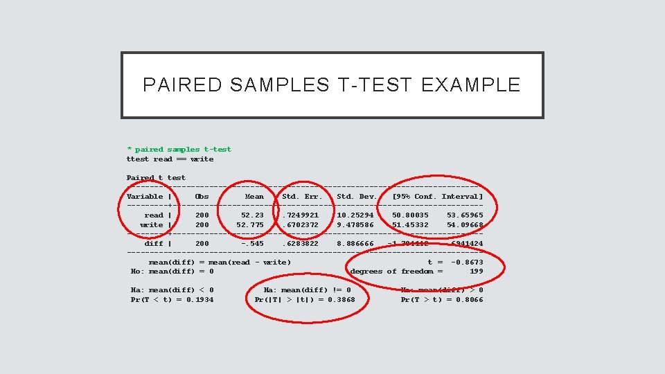
PAIRED SAMPLES T-TEST EXAMPLE * paired samples t-test ttest read == write Paired t test ---------------------------------------Variable | Obs Mean Std. Err. Std. Dev. [95% Conf. Interval] -----+----------------------------------read | 200 52. 23. 7249921 10. 25294 50. 80035 53. 65965 write | 200 52. 775. 6702372 9. 478586 51. 45332 54. 09668 -----+----------------------------------diff | 200 -. 545. 6283822 8. 886666 -1. 784142. 6941424 ---------------------------------------mean(diff) = mean(read - write) t = -0. 8673 Ho: mean(diff) = 0 degrees of freedom = 199 Ha: mean(diff) < 0 Pr(T < t) = 0. 1934 Ha: mean(diff) != 0 Pr(|T| > |t|) = 0. 3868 Ha: mean(diff) > 0 Pr(T > t) = 0. 8066

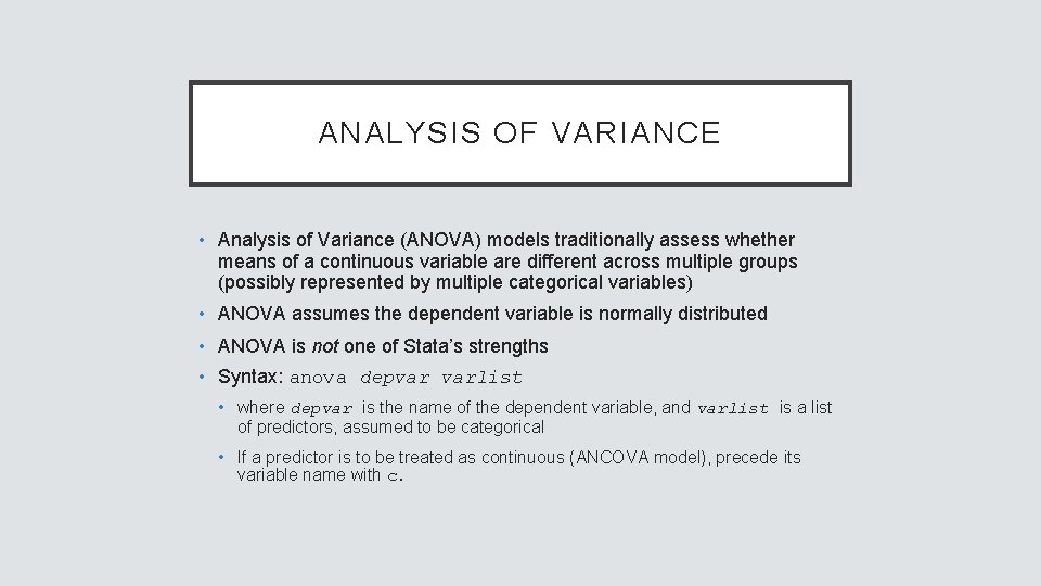
ANALYSIS OF VARIANCE • Analysis of Variance (ANOVA) models traditionally assess whether means of a continuous variable are different across multiple groups (possibly represented by multiple categorical variables) • ANOVA assumes the dependent variable is normally distributed • ANOVA is not one of Stata’s strengths • Syntax: anova depvar varlist • where depvar is the name of the dependent variable, and varlist is a list of predictors, assumed to be categorical • If a predictor is to be treated as continuous (ANCOVA model), precede its variable name with c.

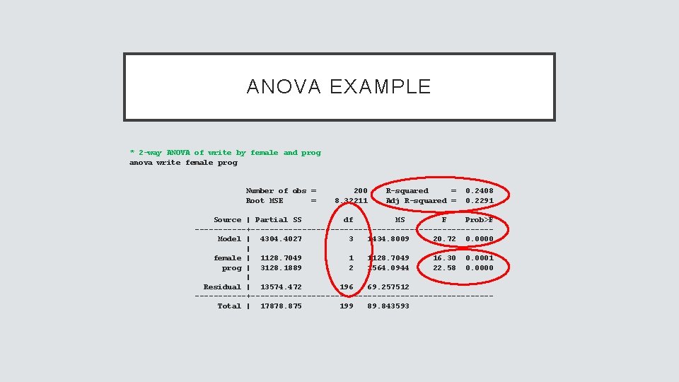
ANOVA EXAMPLE * 2 -way ANOVA of write by female and prog anova write female prog Number of obs = Root MSE = 200 8. 32211 R-squared = Adj R-squared = 0. 2408 0. 2291 Source | Partial SS df MS F Prob>F ------+--------------------------Model | 4304. 4027 3 1434. 8009 20. 72 0. 0000 | female | 1128. 7049 16. 30 0. 0001 prog | 3128. 1889 2 1564. 0944 22. 58 0. 0000 | Residual | 13574. 472 196 69. 257512 ------+--------------------------Total | 17878. 875 199 89. 843593

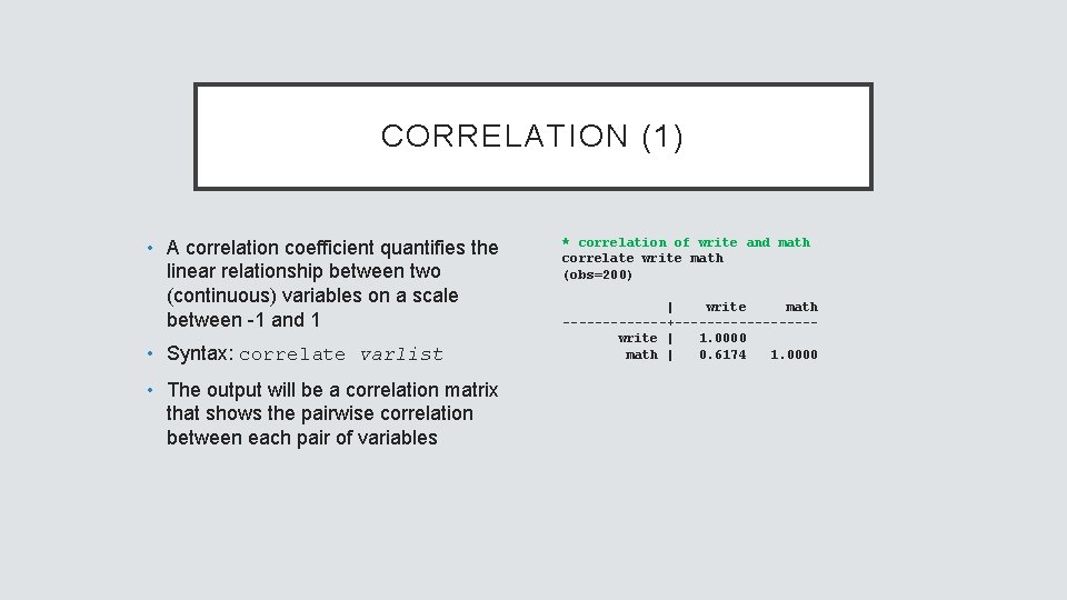
CORRELATION (1) • A correlation coefficient quantifies the linear relationship between two (continuous) variables on a scale between -1 and 1 • Syntax: correlate varlist • The output will be a correlation matrix that shows the pairwise correlation between each pair of variables * correlation of write and math correlate write math (obs=200) | write math -------+---------write | 1. 0000 math | 0. 6174 1. 0000

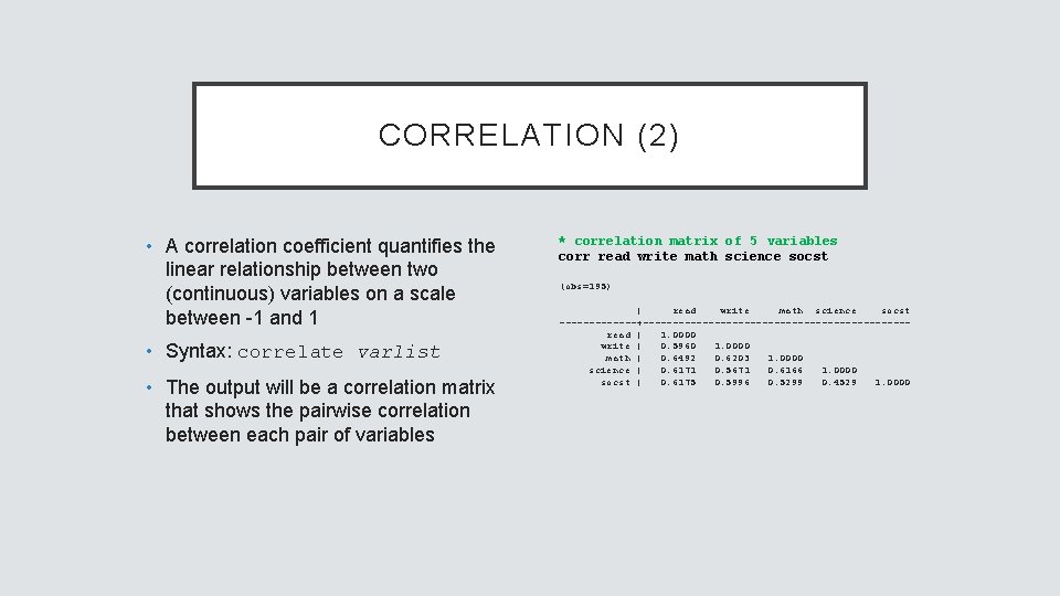
CORRELATION (2) • A correlation coefficient quantifies the linear relationship between two (continuous) variables on a scale between -1 and 1 • Syntax: correlate varlist • The output will be a correlation matrix that shows the pairwise correlation between each pair of variables * correlation matrix of 5 variables corr read write math science socst (obs=195) | read write math science socst -------+----------------------read | 1. 0000 write | 0. 5960 1. 0000 math | 0. 6492 0. 6203 1. 0000 science | 0. 6171 0. 5671 0. 6166 1. 0000 socst | 0. 6175 0. 5996 0. 5299 0. 4529 1. 0000

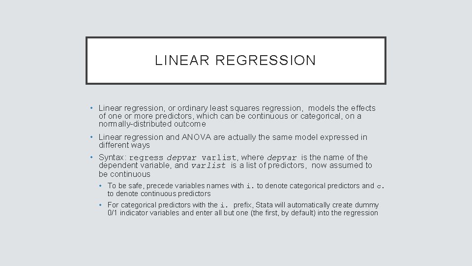
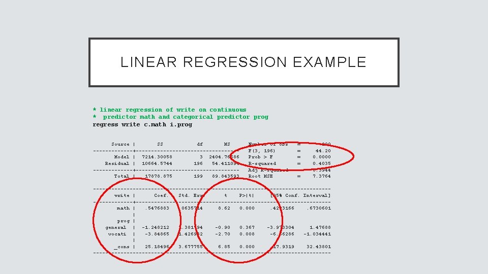
LINEAR REGRESSION • Linear regression, or ordinary least squares regression, models the effects of one or more predictors, which can be continuous or categorical, on a normally-distributed outcome • Linear regression and ANOVA are actually the same model expressed in different ways • Syntax: regress depvar varlist, where depvar is the name of the dependent variable, and varlist is a list of predictors, now assumed to be continuous • To be safe, precede variables names with i. to denote categorical predictors and c. to denote continuous predictors • For categorical predictors with the i. prefix, Stata will automatically create dummy 0/1 indicator variables and enter all but one (the first, by default) into the regression

LINEAR REGRESSION EXAMPLE * linear regression of write on continuous * predictor math and categorical predictor prog regress write c. math i. prog Source | SS df MS -------+-----------------Model | 7214. 30058 3 2404. 76686 Residual | 10664. 5744 196 54. 411094 -------+-----------------Total | 17878. 875 199 89. 843593 Number of obs F(3, 196) Prob > F R-squared Adj R-squared Root MSE = = = 200 44. 20 0. 0000 0. 4035 0. 3944 7. 3764 ---------------------------------------write | Coef. Std. Err. t P>|t| [95% Conf. Interval] -------+--------------------------------math |. 5476883. 0635714 8. 62 0. 000. 4223166. 6730601 | prog | general | -1. 248212 1. 381794 -0. 90 0. 367 -3. 973304 1. 47688 vocati | -3. 84865 1. 426982 -2. 70 0. 008 -6. 66286 -1. 034441 | _cons | 25. 18496 3. 677755 6. 85 0. 000 17. 9319 32. 43801 ---------------------------------------

ESTIMATING STATISTICS BASED ON A MODEL • Stata provides excellent support for estimating and testing additional statistics after a regression model has been run • Stata refers to these as “postestimation” commands, and they can be used after most regression models • Some examples: • Model predictions: predicted outcomes, residuals, influence statistics, etc. • Joint tests of coefficients or linear combination of statistics • Marginal estimates

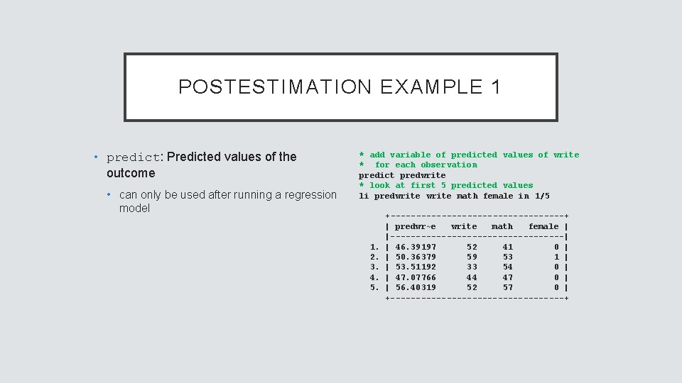
POSTESTIMATION EXAMPLE 1 • predict: Predicted values of the outcome • can only be used after running a regression model * add variable of predicted values of write * for each observation predict predwrite * look at first 5 predicted values li predwrite math female in 1/5 1. 2. 3. 4. 5. +-----------------+ | predwr~e write math female | |-----------------| | 46. 39197 52 41 0 | | 50. 36379 59 53 1 | | 53. 51192 33 54 0 | | 47. 07766 44 47 0 | | 56. 40319 52 57 0 | +-----------------+

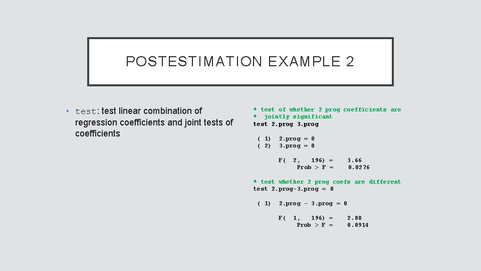
POSTESTIMATION EXAMPLE 2 • test: test linear combination of regression coefficients and joint tests of coefficients * test of whether 2 prog coefficients are * jointly significant test 2. prog 3. prog ( 1) ( 2) 2. prog = 0 3. prog = 0 F( 2, 196) = Prob > F = 3. 66 0. 0276 * test whether 2 prog coefs are different test 2. prog-3. prog = 0 ( 1) 2. prog - 3. prog = 0 F( 1, 196) = Prob > F = 2. 88 0. 0914

ANALYSIS OF CATEGORICAL OUTCOMES tab …, chi 2 chi-square test of independence logit logistic regression

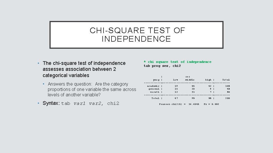
CHI-SQUARE TEST OF INDEPENDENCE • The chi-square test of independence assesses association between 2 categorical variables • Answers the question: Are the category proportions of one variable the same across levels of another variable? • Syntax: tab var 1 var 2, chi 2 * chi square test of independence tab prog ses, chi 2 | ses prog | low middle high | Total ------+-----------------+-----academic | 19 44 42 | 105 general | 16 20 9 | 45 vocati | 12 31 7 | 50 ------+-----------------+-----Total | 47 95 58 | 200 Pearson chi 2(4) = 16. 6044 Pr = 0. 002

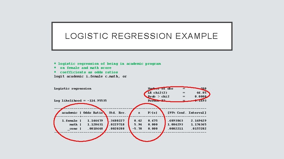
LOGISTIC REGRESSION • Logistic regression is used to estimate the effect of multiple predictors on a binary outcome • Syntax very similar to regress: logit depvar varlist, where depvar is a binary outcome variable and varlist is a list of predictors • Add the or option to output the coefficients as odds ratios

LOGISTIC REGRESSION EXAMPLE * logistic regression of being in academic program * on female and math score * coefficients as odds ratios logit academic i. female c. math, or Logistic regression Log likelihood = -114. 95535 Number of obs LR chi 2(2) Prob > chi 2 Pseudo R 2 = = 200 46. 85 0. 0000 0. 1693 ---------------------------------------academic | Odds Ratio Std. Err. z P>|z| [95% Conf. Interval] -------+--------------------------------1. female | 1. 144479. 3680227 0. 42 0. 675. 6093863 2. 149429 math | 1. 128431. 0229718 5. 94 0. 000 1. 084293 1. 174365 _cons |. 0018648. 0020288 -5. 78 0. 0002211. 0157282 ---------------------------------------

ADDITIONAL RESOURCES FOR LEARNING STATA

IDRE STATISTICAL CONSULTING WEBSITE • The IDRE Statistical Consulting website is a well-known resource for coding support for several statistical software packages • https: //stats. idre. ucla. edu • Stata was beloved by previous members of the group, so Stata is particularly well represented on our website

IDRE STATISTICAL CONSULTING WEBSITE STATA PAGES • On the website landing page for Stata, you’ll find many links to our Stata resources pages • https: //stats. idre. ucla. edu/stata/ • These resources include: • seminars, deeper dives into Stata topics that are often delivered live on campus • learning modules for basic Stata commands • data analysis examples of many different regression commands • annotated output of many regression commands

EXTERNAL RESOURCES • Stata You. Tube channel (run by Stata. Corp) • Stata FAQ (compiled by Stata. Corp) • Stata cheat sheets (compact guides to Stata commands)

END THANK YOU!