Introduction to SQL 1 Why SQL SQL is

Introduction to SQL 1

Why SQL? • SQL is a very-high-level language, in which the programmer is able to avoid specifying a lot of data-manipulation details that would be necessary in other languages. • What makes SQL viable is that its queries are “optimized” quite well, yielding efficient query executions. 2

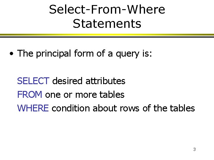
Select-From-Where Statements • The principal form of a query is: SELECT desired attributes FROM one or more tables WHERE condition about rows of the tables 3

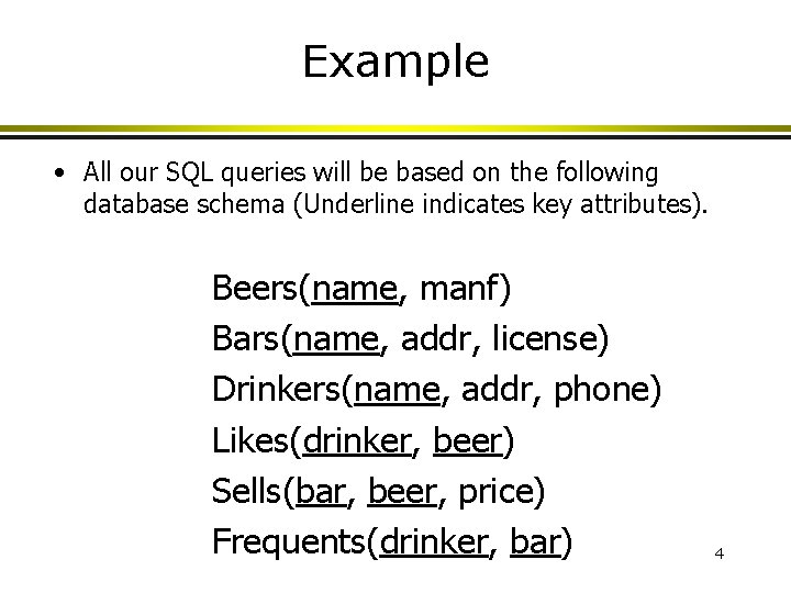
Example • All our SQL queries will be based on the following database schema (Underline indicates key attributes). Beers(name, manf) Bars(name, addr, license) Drinkers(name, addr, phone) Likes(drinker, beer) Sells(bar, beer, price) Frequents(drinker, bar) 4

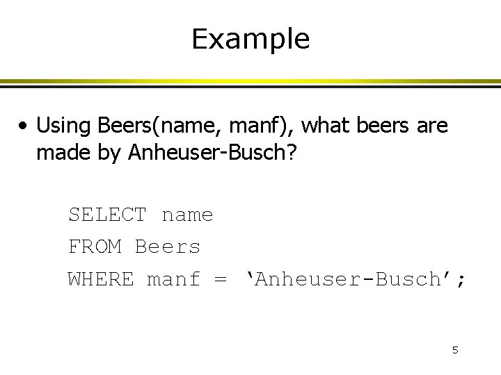
Example • Using Beers(name, manf), what beers are made by Anheuser-Busch? SELECT name FROM Beers WHERE manf = ‘Anheuser-Busch’; 5

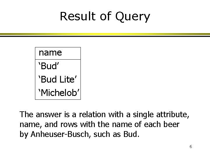
Result of Query name ‘Bud’ ‘Bud Lite’ ‘Michelob’ The answer is a relation with a single attribute, name, and rows with the name of each beer by Anheuser-Busch, such as Bud. 6

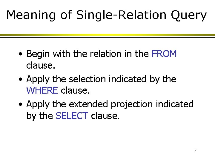
Meaning of Single-Relation Query • Begin with the relation in the FROM clause. • Apply the selection indicated by the WHERE clause. • Apply the extended projection indicated by the SELECT clause. 7

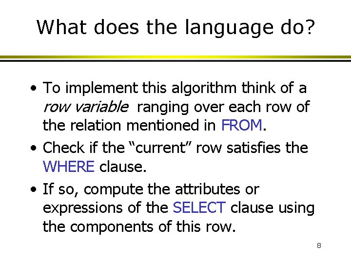
What does the language do? • To implement this algorithm think of a row variable ranging over each row of the relation mentioned in FROM. • Check if the “current” row satisfies the WHERE clause. • If so, compute the attributes or expressions of the SELECT clause using the components of this row. 8

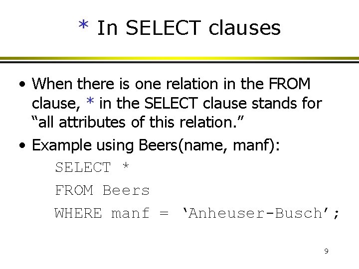
* In SELECT clauses • When there is one relation in the FROM clause, * in the SELECT clause stands for “all attributes of this relation. ” • Example using Beers(name, manf): SELECT * FROM Beers WHERE manf = ‘Anheuser-Busch’; 9

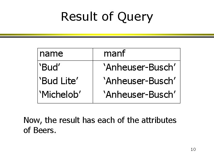
Result of Query name ‘Bud’ ‘Bud Lite’ ‘Michelob’ manf ‘Anheuser-Busch’ Now, the result has each of the attributes of Beers. 10

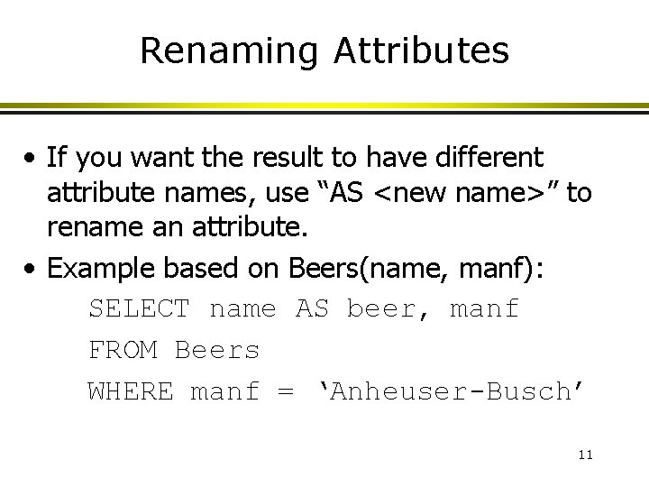
Renaming Attributes • If you want the result to have different attribute names, use “AS <new name>” to rename an attribute. • Example based on Beers(name, manf): SELECT name AS beer, manf FROM Beers WHERE manf = ‘Anheuser-Busch’ 11

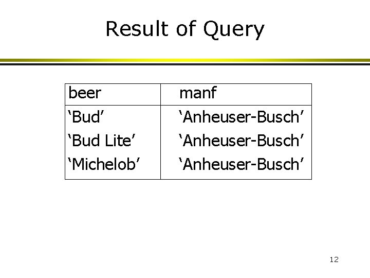
Result of Query beer ‘Bud’ ‘Bud Lite’ ‘Michelob’ manf ‘Anheuser-Busch’ 12

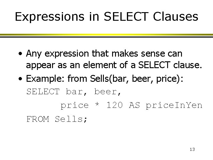
Expressions in SELECT Clauses • Any expression that makes sense can appear as an element of a SELECT clause. • Example: from Sells(bar, beer, price): SELECT bar, beer, price * 120 AS price. In. Yen FROM Sells; 13

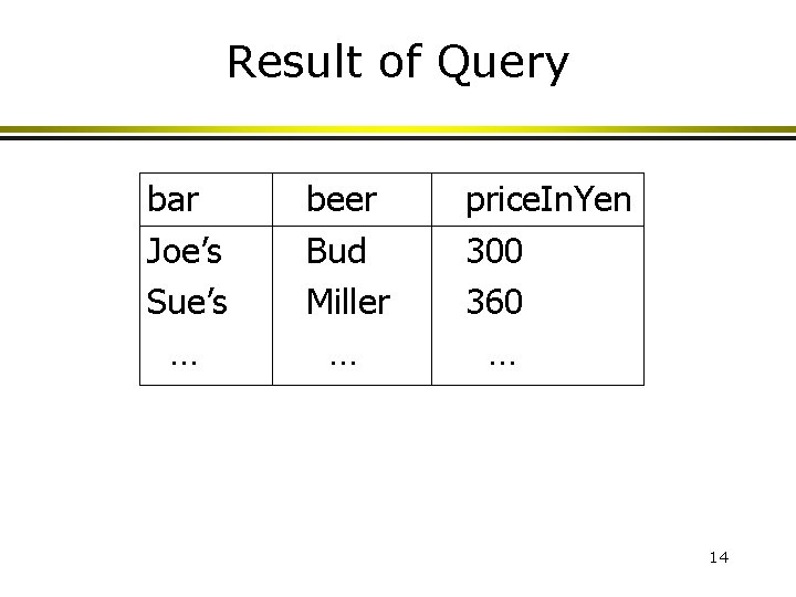
Result of Query bar Joe’s Sue’s … beer Bud Miller … price. In. Yen 300 360 … 14

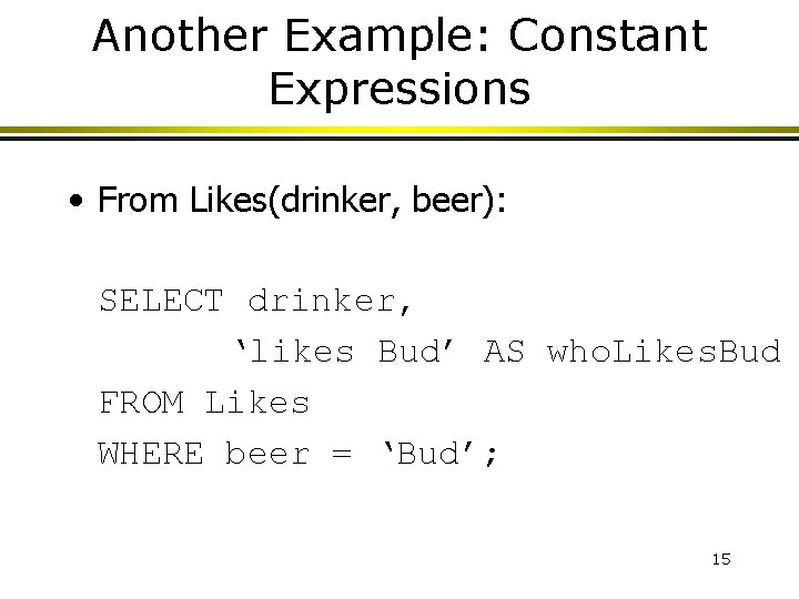
Another Example: Constant Expressions • From Likes(drinker, beer): SELECT drinker, ‘likes Bud’ AS who. Likes. Bud FROM Likes WHERE beer = ‘Bud’; 15

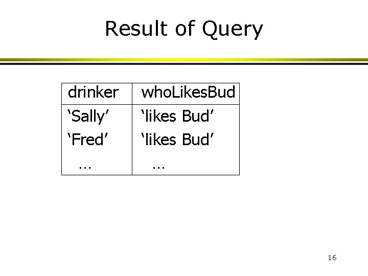
Result of Query drinker ‘Sally’ ‘Fred’ … who. Likes. Bud ‘likes Bud’ … 16

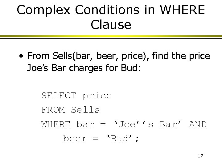
Complex Conditions in WHERE Clause • From Sells(bar, beer, price), find the price Joe’s Bar charges for Bud: SELECT price FROM Sells WHERE bar = ‘Joe’’s Bar’ AND beer = ‘Bud’; 17

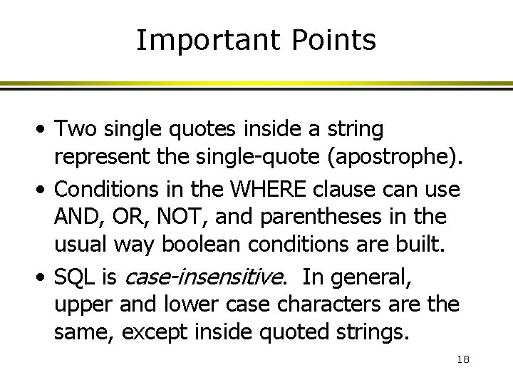
Important Points • Two single quotes inside a string represent the single-quote (apostrophe). • Conditions in the WHERE clause can use AND, OR, NOT, and parentheses in the usual way boolean conditions are built. • SQL is case-insensitive. In general, upper and lower case characters are the same, except inside quoted strings. 18

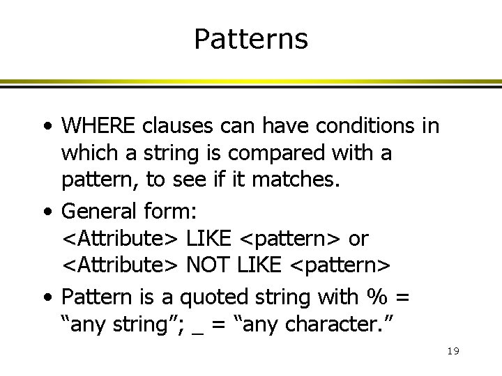
Patterns • WHERE clauses can have conditions in which a string is compared with a pattern, to see if it matches. • General form: <Attribute> LIKE <pattern> or <Attribute> NOT LIKE <pattern> • Pattern is a quoted string with % = “any string”; _ = “any character. ” 19

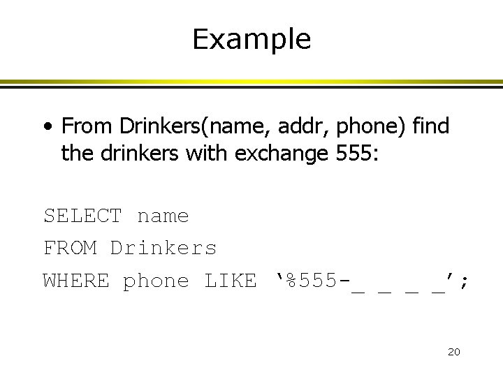
Example • From Drinkers(name, addr, phone) find the drinkers with exchange 555: SELECT name FROM Drinkers WHERE phone LIKE ‘%555 -_ _ _ _’; 20

NULL Values • Rows in SQL relations can have NULL as a value for one or more components. • Meaning depends on context. Two common cases: • Missing value : e. g. , we know Joe’s Bar has some address, but we don’t know what it is. • Inapplicable : e. g. , the value of attribute spouse for an unmarried person. 21

Comparing NULL’s to Values • The logic of conditions in SQL is really 3 valued logic: TRUE, FALSE, UNKNOWN. • When any value is compared with NULL, the truth value is UNKNOWN. • But a query only produces a row in the answer if its truth value for the WHERE clause is TRUE (not FALSE or UNKNOWN). 22

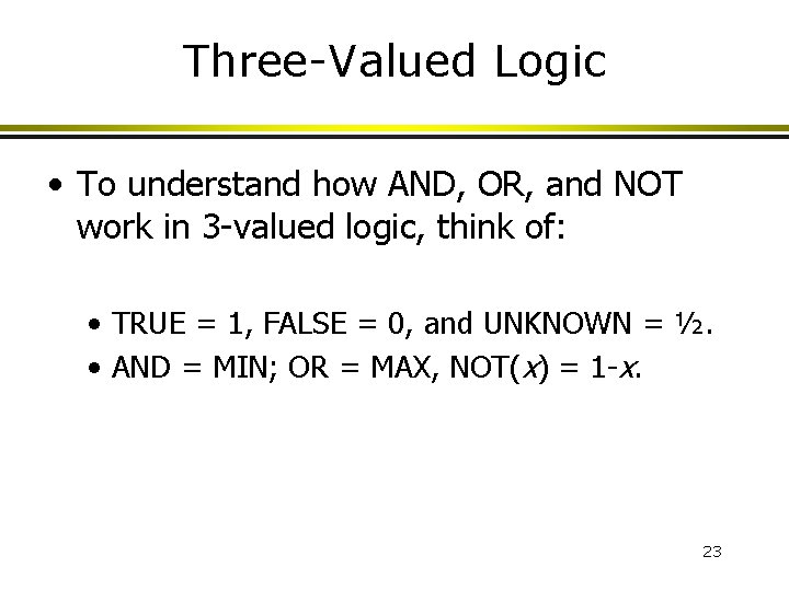
Three-Valued Logic • To understand how AND, OR, and NOT work in 3 -valued logic, think of: • TRUE = 1, FALSE = 0, and UNKNOWN = ½. • AND = MIN; OR = MAX, NOT(x) = 1 -x. 23

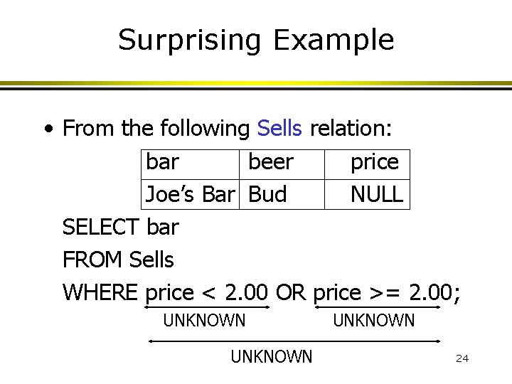
Surprising Example • From the following Sells relation: bar beer price Joe’s Bar Bud NULL SELECT bar FROM Sells WHERE price < 2. 00 OR price >= 2. 00; UNKNOWN 24

Reason: 2 -Valued Laws != 3 Valued Laws • Some common laws, like the commutatively of AND, hold in 3 -valued logic. • But others do not; example: the “law of excluded middle, ” p OR NOT p = TRUE. 25

Multi-relation Queries • Interesting queries often combine data from more than one relation. • We can address several relations in one query by listing them all in the FROM clause. • Distinguish attributes of the same name by “<relation>. <attribute>” 26

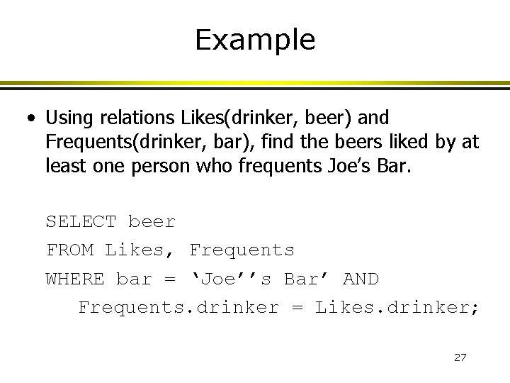
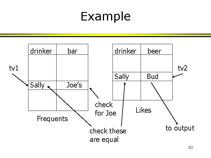
Example • Using relations Likes(drinker, beer) and Frequents(drinker, bar), find the beers liked by at least one person who frequents Joe’s Bar. SELECT beer FROM Likes, Frequents WHERE bar = ‘Joe’’s Bar’ AND Frequents. drinker = Likes. drinker; 27

Formal Semantics Almost the same as for single-relation queries: 1. Start with the product of all the relations in the FROM clause. 2. Apply the selection condition from the WHERE clause. 3. Project onto the list of attributes and expressions in the SELECT clause. 28

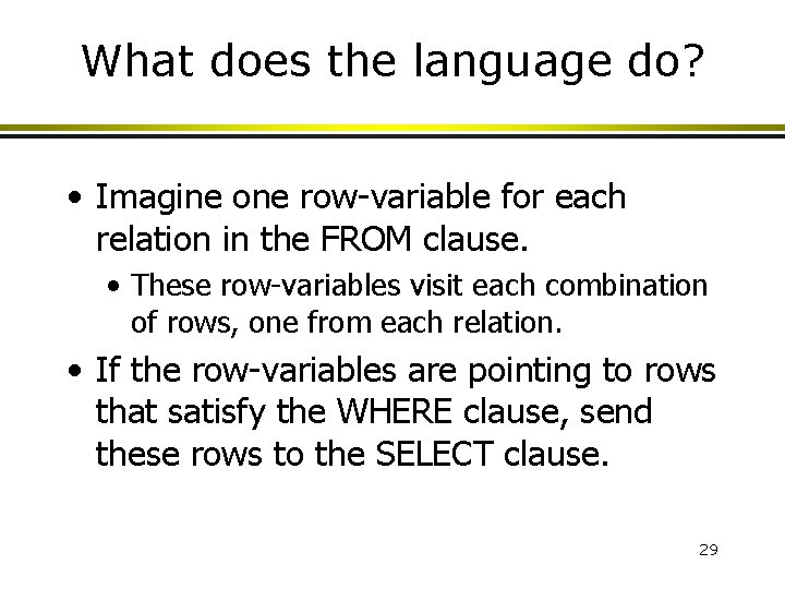
What does the language do? • Imagine one row-variable for each relation in the FROM clause. • These row-variables visit each combination of rows, one from each relation. • If the row-variables are pointing to rows that satisfy the WHERE clause, send these rows to the SELECT clause. 29

Example drinker bar tv 1 Sally Joe’s Frequents drinker Sally check for Joe check these are equal beer Bud tv 2 Likes to output 30

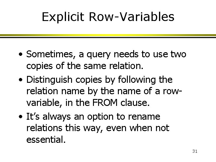
Explicit Row-Variables • Sometimes, a query needs to use two copies of the same relation. • Distinguish copies by following the relation name by the name of a rowvariable, in the FROM clause. • It’s always an option to rename relations this way, even when not essential. 31

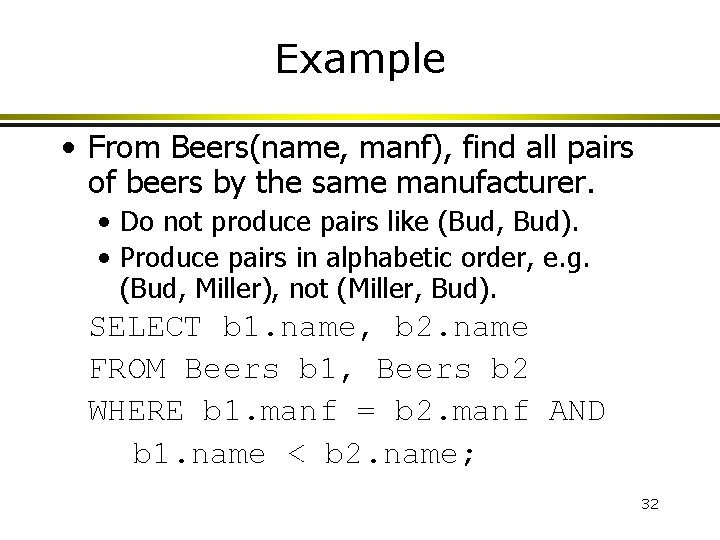
Example • From Beers(name, manf), find all pairs of beers by the same manufacturer. • Do not produce pairs like (Bud, Bud). • Produce pairs in alphabetic order, e. g. (Bud, Miller), not (Miller, Bud). SELECT b 1. name, b 2. name FROM Beers b 1, Beers b 2 WHERE b 1. manf = b 2. manf AND b 1. name < b 2. name; 32

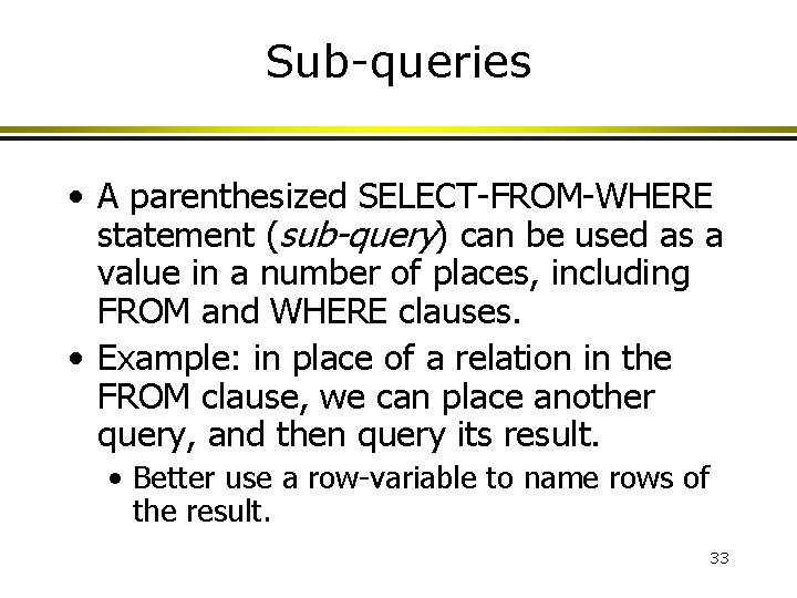
Sub-queries • A parenthesized SELECT-FROM-WHERE statement (sub-query) can be used as a value in a number of places, including FROM and WHERE clauses. • Example: in place of a relation in the FROM clause, we can place another query, and then query its result. • Better use a row-variable to name rows of the result. 33

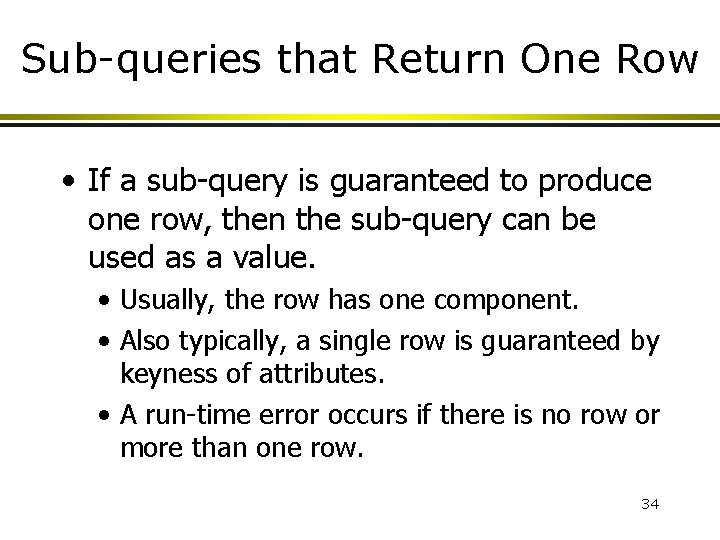
Sub-queries that Return One Row • If a sub-query is guaranteed to produce one row, then the sub-query can be used as a value. • Usually, the row has one component. • Also typically, a single row is guaranteed by keyness of attributes. • A run-time error occurs if there is no row or more than one row. 34

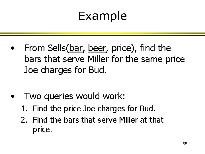
Example • From Sells(bar, beer, price), find the bars that serve Miller for the same price Joe charges for Bud. • Two queries would work: 1. Find the price Joe charges for Bud. 2. Find the bars that serve Miller at that price. 35

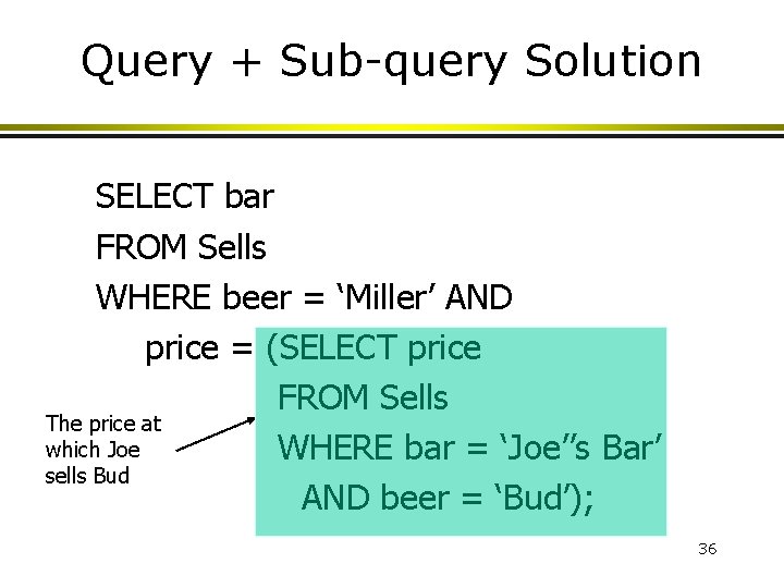
Query + Sub-query Solution SELECT bar FROM Sells WHERE beer = ‘Miller’ AND price = (SELECT price FROM Sells The price at which Joe WHERE bar = ‘Joe’’s Bar’ sells Bud AND beer = ‘Bud’); 36

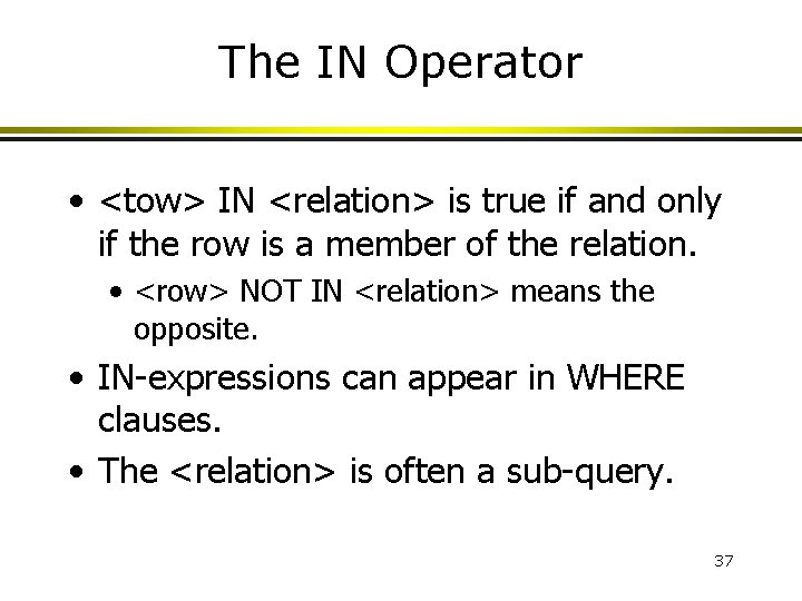
The IN Operator • <tow> IN <relation> is true if and only if the row is a member of the relation. • <row> NOT IN <relation> means the opposite. • IN-expressions can appear in WHERE clauses. • The <relation> is often a sub-query. 37

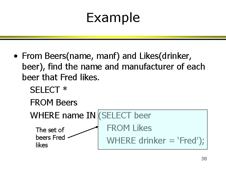
Example • From Beers(name, manf) and Likes(drinker, beer), find the name and manufacturer of each beer that Fred likes. SELECT * FROM Beers WHERE name IN (SELECT beer FROM Likes The set of beers Fred WHERE drinker = ‘Fred’); likes 38

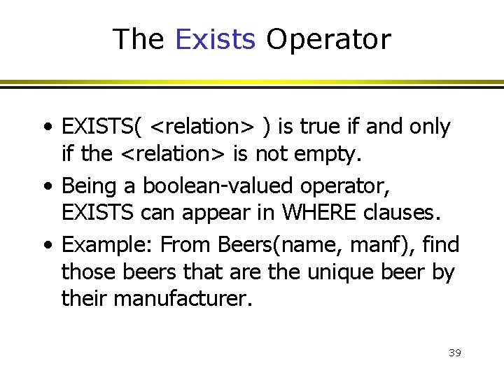
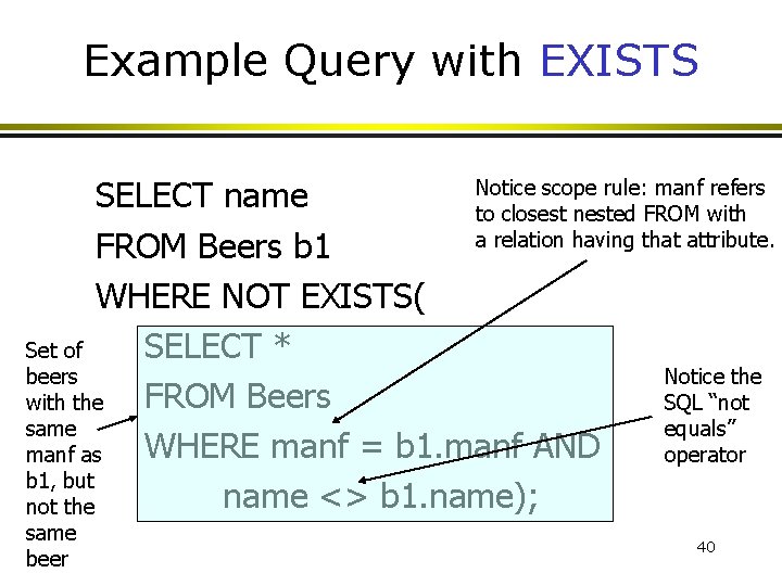
The Exists Operator • EXISTS( <relation> ) is true if and only if the <relation> is not empty. • Being a boolean-valued operator, EXISTS can appear in WHERE clauses. • Example: From Beers(name, manf), find those beers that are the unique beer by their manufacturer. 39

Example Query with EXISTS Notice scope rule: manf refers SELECT name to closest nested FROM with a relation having that attribute. FROM Beers b 1 WHERE NOT EXISTS( SELECT * Set of beers Notice the FROM Beers SQL “not with the same equals” WHERE manf = b 1. manf AND manf as operator b 1, but name <> b 1. name); not the same beer 40

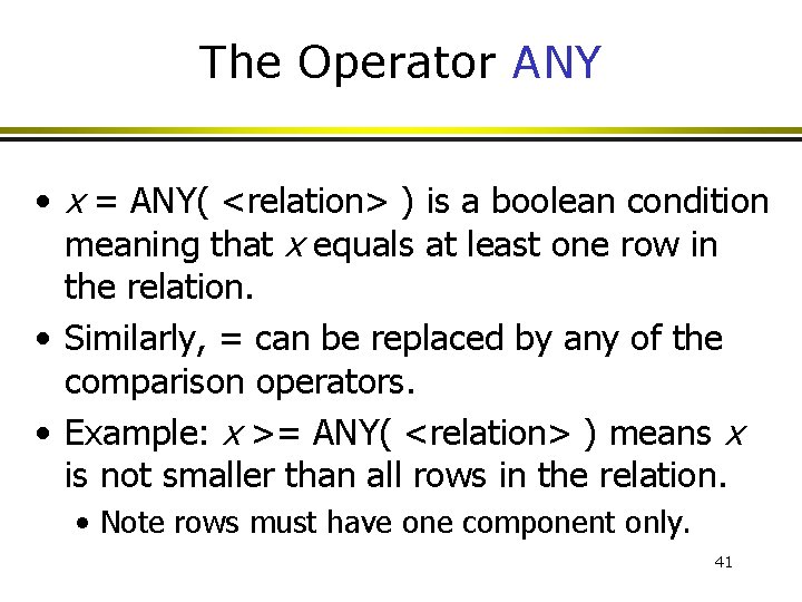
The Operator ANY • x = ANY( <relation> ) is a boolean condition meaning that x equals at least one row in the relation. • Similarly, = can be replaced by any of the comparison operators. • Example: x >= ANY( <relation> ) means x is not smaller than all rows in the relation. • Note rows must have one component only. 41

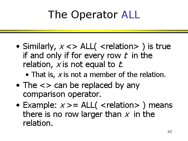
The Operator ALL • Similarly, x <> ALL( <relation> ) is true if and only if for every row t in the relation, x is not equal to t. • That is, x is not a member of the relation. • The <> can be replaced by any comparison operator. • Example: x >= ALL( <relation> ) means there is no row larger than x in the relation. 42

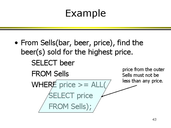
Example • From Sells(bar, beer, price), find the beer(s) sold for the highest price. SELECT beer price from the outer FROM Sells must not be less than any price. WHERE price >= ALL( SELECT price FROM Sells); 43

More SQL? Relations as Bags Grouping and Aggregation Database Modification 44

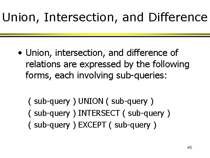
Union, Intersection, and Difference • Union, intersection, and difference of relations are expressed by the following forms, each involving sub-queries: ( sub-query ) UNION ( sub-query ) INTERSECT ( sub-query ) EXCEPT ( sub-query ) 45

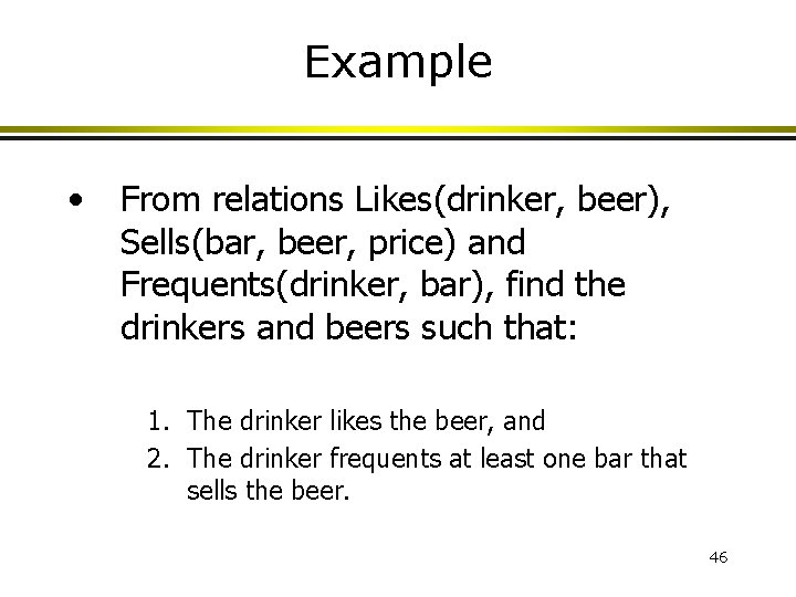
Example • From relations Likes(drinker, beer), Sells(bar, beer, price) and Frequents(drinker, bar), find the drinkers and beers such that: 1. The drinker likes the beer, and 2. The drinker frequents at least one bar that sells the beer. 46

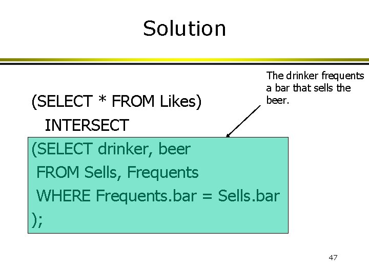
Solution The drinker frequents a bar that sells the beer. (SELECT * FROM Likes) INTERSECT (SELECT drinker, beer FROM Sells, Frequents WHERE Frequents. bar = Sells. bar ); 47

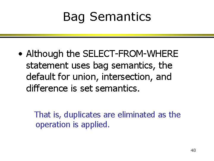
Bag Semantics • Although the SELECT-FROM-WHERE statement uses bag semantics, the default for union, intersection, and difference is set semantics. That is, duplicates are eliminated as the operation is applied. 48

Motivation: Efficiency • When doing projection in relational algebra, it is easier to avoid eliminating duplicates. • Just work row-at-a-time. • When doing intersection or difference, it is most efficient to sort the relations first. • At that point you may as well eliminate the duplicates anyway. 49

Controlling Duplicate Elimination • Force the result to be a set by SELECT DISTINCT. . . • Force the result to be a bag (i. e. , don’t eliminate duplicates) by ALL, as in. . . UNION ALL. . . 50

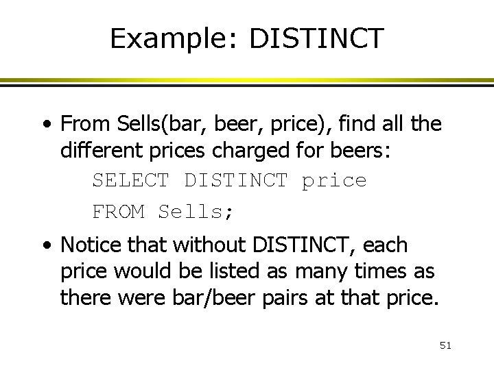
Example: DISTINCT • From Sells(bar, beer, price), find all the different prices charged for beers: SELECT DISTINCT price FROM Sells; • Notice that without DISTINCT, each price would be listed as many times as there were bar/beer pairs at that price. 51

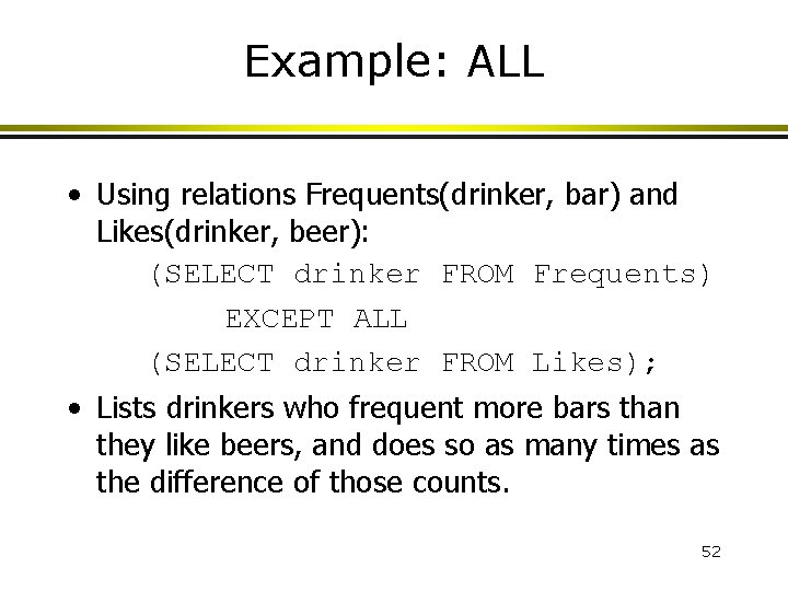
Example: ALL • Using relations Frequents(drinker, bar) and Likes(drinker, beer): (SELECT drinker FROM Frequents) EXCEPT ALL (SELECT drinker FROM Likes); • Lists drinkers who frequent more bars than they like beers, and does so as many times as the difference of those counts. 52

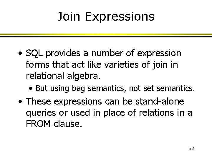
Join Expressions • SQL provides a number of expression forms that act like varieties of join in relational algebra. • But using bag semantics, not semantics. • These expressions can be stand-alone queries or used in place of relations in a FROM clause. 53

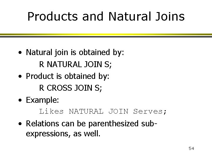
Products and Natural Joins • Natural join is obtained by: R NATURAL JOIN S; • Product is obtained by: R CROSS JOIN S; • Example: Likes NATURAL JOIN Serves; • Relations can be parenthesized subexpressions, as well. 54

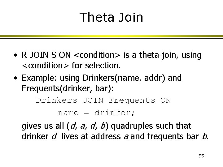
Theta Join • R JOIN S ON <condition> is a theta-join, using <condition> for selection. • Example: using Drinkers(name, addr) and Frequents(drinker, bar): Drinkers JOIN Frequents ON name = drinker; gives us all (d, a, d, b) quadruples such that drinker d lives at address a and frequents bar b. 55

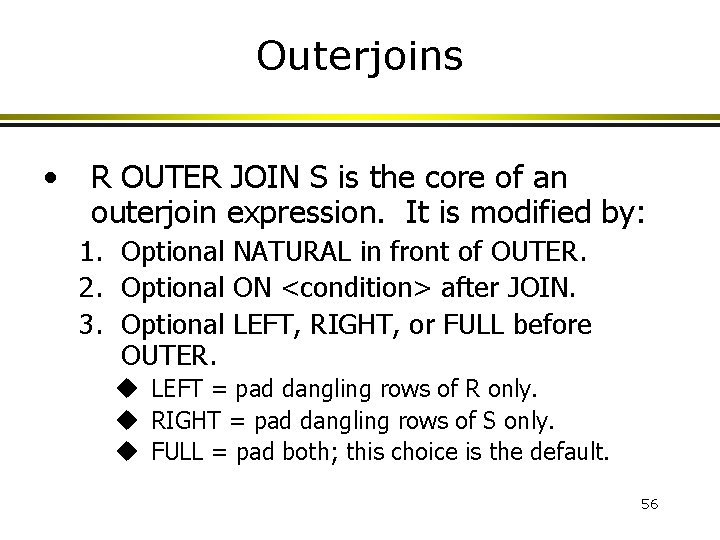
Outerjoins • R OUTER JOIN S is the core of an outerjoin expression. It is modified by: 1. Optional NATURAL in front of OUTER. 2. Optional ON <condition> after JOIN. 3. Optional LEFT, RIGHT, or FULL before OUTER. u LEFT = pad dangling rows of R only. u RIGHT = pad dangling rows of S only. u FULL = pad both; this choice is the default. 56

Aggregations • SUM, AVG, COUNT, MIN, and MAX can be applied to a column in a SELECT clause to produce that aggregation on the column. • Also, COUNT(*) counts the number of rows. 57

Example: Aggregation • From Sells(bar, beer, price), find the average price of Bud: SELECT AVG(price) FROM Sells WHERE beer = ‘Bud’; 58

Eliminating Duplicates in an Aggregation • DISTINCT inside an aggregation causes duplicates to be eliminated before the aggregation. • Example: find the number of different prices charged for Bud: SELECT COUNT(DISTINCT price) FROM Sells WHERE beer = ‘Bud’; 59

NULL’s Ignored in Aggregation • NULL never contributes to a sum, average, or count, and can never be the minimum or maximum of a column. • But if there are no non-NULL values in a column, then the result of the aggregation is NULL. 60

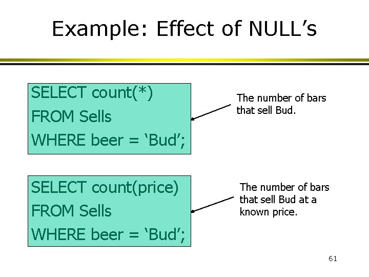
Example: Effect of NULL’s SELECT count(*) FROM Sells WHERE beer = ‘Bud’; SELECT count(price) FROM Sells WHERE beer = ‘Bud’; The number of bars that sell Bud at a known price. 61

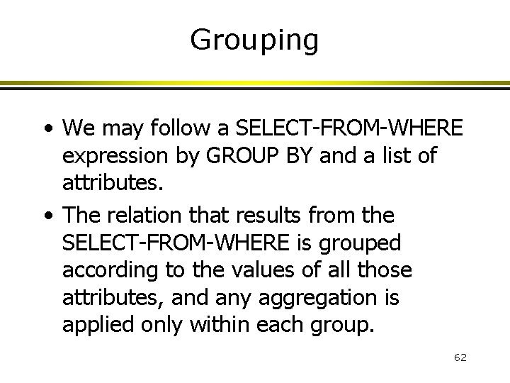
Grouping • We may follow a SELECT-FROM-WHERE expression by GROUP BY and a list of attributes. • The relation that results from the SELECT-FROM-WHERE is grouped according to the values of all those attributes, and any aggregation is applied only within each group. 62

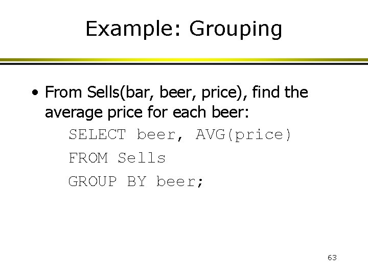
Example: Grouping • From Sells(bar, beer, price), find the average price for each beer: SELECT beer, AVG(price) FROM Sells GROUP BY beer; 63

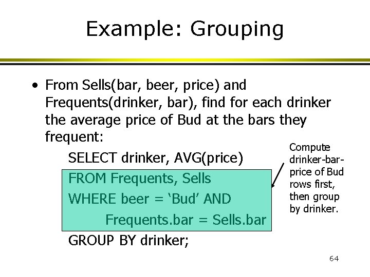
Example: Grouping • From Sells(bar, beer, price) and Frequents(drinker, bar), find for each drinker the average price of Bud at the bars they frequent: Compute SELECT drinker, AVG(price) drinker-barprice of Bud FROM Frequents, Sells rows first, then group WHERE beer = ‘Bud’ AND by drinker. Frequents. bar = Sells. bar GROUP BY drinker; 64

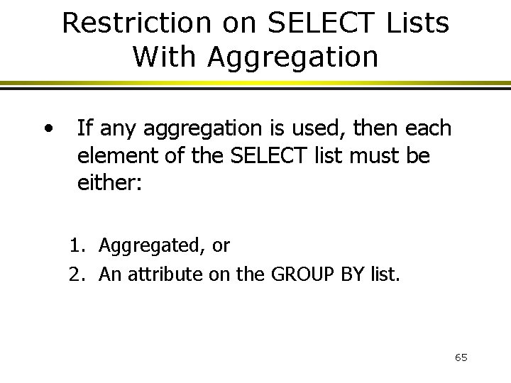
Restriction on SELECT Lists With Aggregation • If any aggregation is used, then each element of the SELECT list must be either: 1. Aggregated, or 2. An attribute on the GROUP BY list. 65

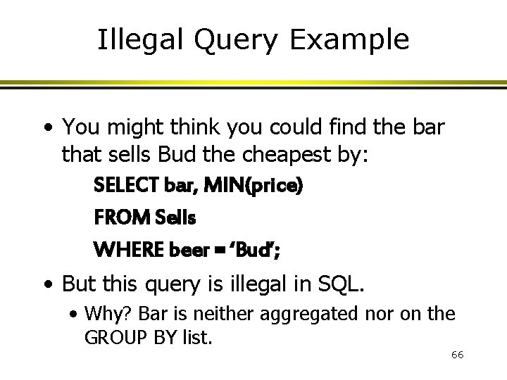
Illegal Query Example • You might think you could find the bar that sells Bud the cheapest by: SELECT bar, MIN(price) FROM Sells WHERE beer = ‘Bud’; • But this query is illegal in SQL. • Why? Bar is neither aggregated nor on the GROUP BY list. 66

HAVING Clauses • HAVING <condition> may follow a GROUP BY clause. • If so, the condition applies to each group, and groups not satisfying the condition are eliminated. 67

Requirements on HAVING Conditions • • These conditions may refer to any relation or row-variable in the FROM clause. They may refer to attributes of those relations, as long as the attribute makes sense within a group; i. e. , it is either: 1. A grouping attribute, or 2. Aggregated. 68

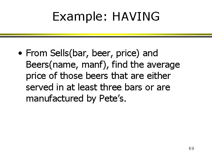
Example: HAVING • From Sells(bar, beer, price) and Beers(name, manf), find the average price of those beers that are either served in at least three bars or are manufactured by Pete’s. 69

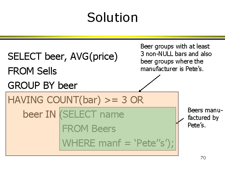
Solution Beer groups with at least 3 non-NULL bars and also beer groups where the manufacturer is Pete’s. SELECT beer, AVG(price) FROM Sells GROUP BY beer HAVING COUNT(bar) >= 3 OR beer IN (SELECT name FROM Beers WHERE manf = ‘Pete’’s’); Beers manufactured by Pete’s. 70

Database Modifications • • A modification command does not return a result as a query does, but it changes the database in some way. There are three kinds of modifications: 1. Insert a row or rows. 2. Delete a row or rows. 3. Update the value(s) of an existing row or rows. 71

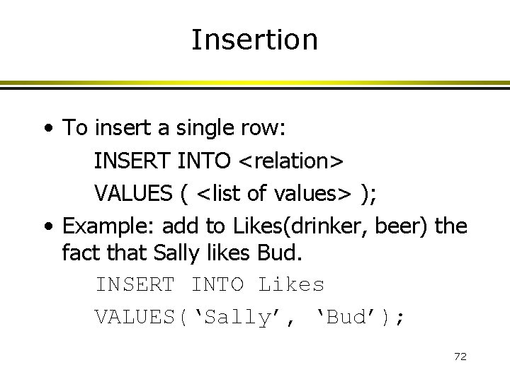
Insertion • To insert a single row: INSERT INTO <relation> VALUES ( <list of values> ); • Example: add to Likes(drinker, beer) the fact that Sally likes Bud. INSERT INTO Likes VALUES(‘Sally’, ‘Bud’); 72

Specifying Attributes in INSERT • • We may add to the relation name a list of attributes. There are two reasons to do so: 1. We forget the standard order of attributes for the relation. 2. We don’t have values for all attributes, and we want the system to fill in missing components with NULL or a default value. 73

Example: Specifying Attributes • Another way to add the fact that Sally likes Bud to Likes(drinker, beer): INSERT INTO Likes(beer, drinker) VALUES(‘Bud’, ‘Sally’); 74

Inserting Many Rows • We may insert the entire result of a query into a relation, using the form: INSERT INTO <relation> ( <sub-query> ); 75

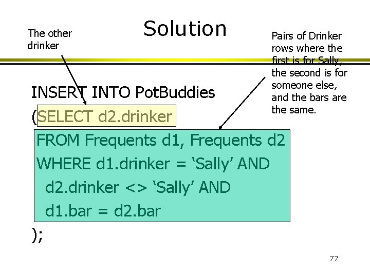
Example: Insert a Sub-query • Using Frequents(drinker, bar), enter into the new relation Pot. Buddies(name) all of Sally’s “potential buddies, ” i. e. , those drinkers who frequent at least one bar that Sally also frequents. 76

The other drinker Solution Pairs of Drinker rows where the first is for Sally, the second is for someone else, and the bars are the same. INSERT INTO Pot. Buddies (SELECT d 2. drinker FROM Frequents d 1, Frequents d 2 WHERE d 1. drinker = ‘Sally’ AND d 2. drinker <> ‘Sally’ AND d 1. bar = d 2. bar ); 77

Deletion • To delete rows satisfying a condition from some relation: DELETE FROM <relation> WHERE <condition>; 78

Example: Deletion • Delete from Likes(drinker, beer) the fact that Sally likes Bud: DELETE FROM Likes WHERE drinker = ‘Sally’ AND beer = ‘Bud’; 79

Example: Delete all Rows • Make the relation Likes empty: DELETE FROM Likes; • Note no WHERE clause needed. 80

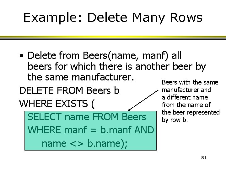
Example: Delete Many Rows • Delete from Beers(name, manf) all beers for which there is another beer by the same manufacturer. Beers with the same manufacturer and DELETE FROM Beers b a different name WHERE EXISTS ( from the name of the beer represented SELECT name FROM Beers by row b. WHERE manf = b. manf AND name <> b. name); 81

Semantics of Deletion -- 1 • Suppose Anheuser-Busch makes only Bud and Bud Light. • Suppose we come to the row b for Bud first. • The sub-query is nonempty, because of the Bud Light row, so we delete Bud. • Now, When b is the row for Bud Light, do we delete that row too? 82

Semantics of Deletion -- 2 • • The answer is that we do delete Bud Light as well. The reason is that deletion proceeds in two stages: 1. Mark all rows for which the WHERE condition is satisfied in the original relation. 2. Delete the marked rows. 83

Updates • To change certain attributes in certain rows of a relation: UPDATE <relation> SET <list of attribute assignments> WHERE <condition on rows>; 84

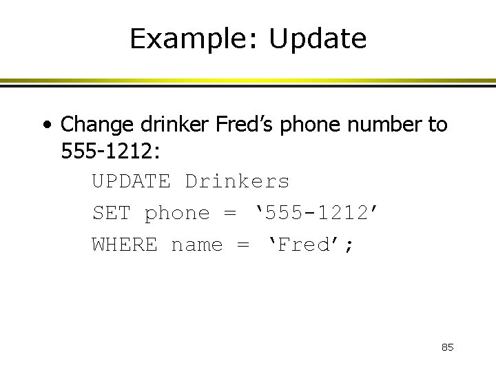
Example: Update • Change drinker Fred’s phone number to 555 -1212: UPDATE Drinkers SET phone = ‘ 555 -1212’ WHERE name = ‘Fred’; 85

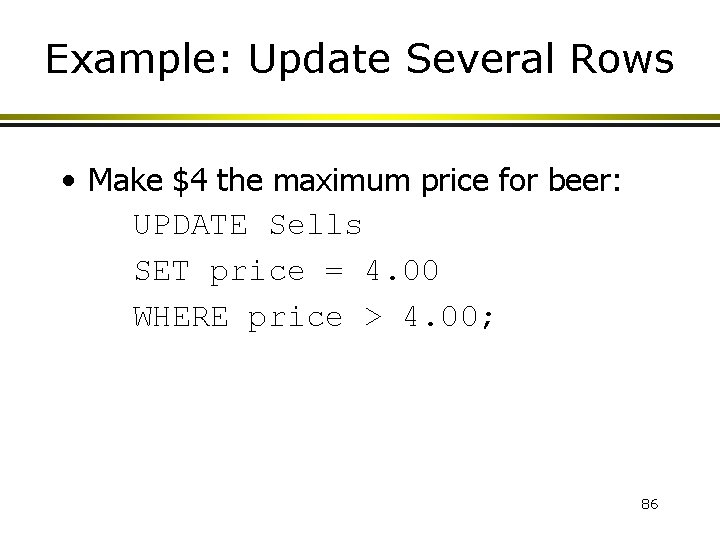
Example: Update Several Rows • Make $4 the maximum price for beer: UPDATE Sells SET price = 4. 00 WHERE price > 4. 00; 86

More SQL? Defining Database Schema Views 87

Defining a Database Schema • A database schema comprises declarations for the relations (“tables”) of the database. • Many other kinds of elements may also appear in the database schema, including views, indexes, and triggers, which we’ll introduce later. 88

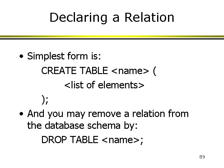
Declaring a Relation • Simplest form is: CREATE TABLE <name> ( <list of elements> ); • And you may remove a relation from the database schema by: DROP TABLE <name>; 89

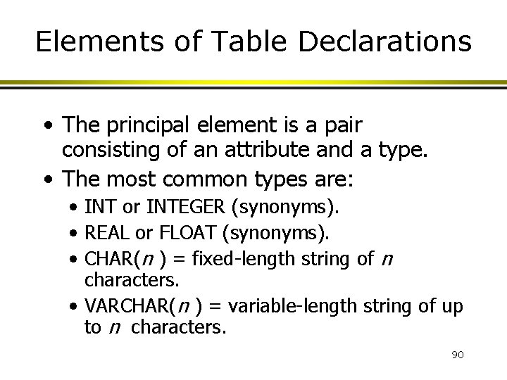
Elements of Table Declarations • The principal element is a pair consisting of an attribute and a type. • The most common types are: • INT or INTEGER (synonyms). • REAL or FLOAT (synonyms). • CHAR(n ) = fixed-length string of n characters. • VARCHAR(n ) = variable-length string of up to n characters. 90

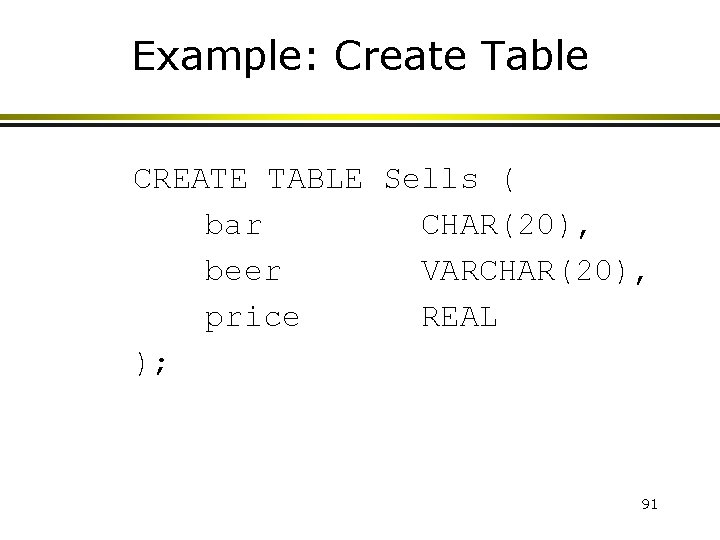
Example: Create Table CREATE TABLE Sells ( bar CHAR(20), beer VARCHAR(20), price REAL ); 91

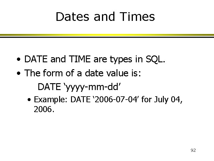
Dates and Times • DATE and TIME are types in SQL. • The form of a date value is: DATE ‘yyyy-mm-dd’ • Example: DATE ‘ 2006 -07 -04’ for July 04, 2006. 92

Times as Values • The form of a time value is: TIME ‘hh: mm: ss’ with an optional decimal point and fractions of a second following. • Example: TIME ’ 15: 30: 02. 5’ = two and a half seconds after 3: 30 PM. 93

Declaring Keys • An attribute or list of attributes may be declared PRIMARY KEY or UNIQUE. • These each say the attribute(s) so declared functionally determine all the attributes of the relation schema. • There a few distinctions to be mentioned later. 94

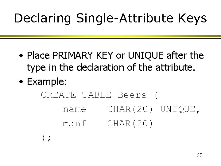
Declaring Single-Attribute Keys • Place PRIMARY KEY or UNIQUE after the type in the declaration of the attribute. • Example: CREATE TABLE Beers ( name CHAR(20) UNIQUE, manf CHAR(20) ); 95

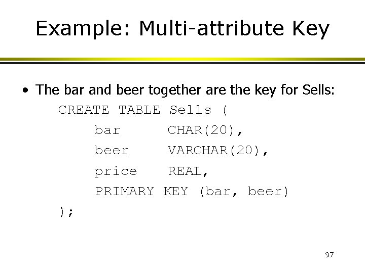
Declaring Multi-attribute Keys • A key declaration can also be another element in the list of elements of a CREATE TABLE statement. • This form is essential if the key consists of more than one attribute. • May be used even for one-attribute keys. 96

Example: Multi-attribute Key • The bar and beer together are the key for Sells: CREATE TABLE Sells ( bar CHAR(20), beer VARCHAR(20), price REAL, PRIMARY KEY (bar, beer) ); 97

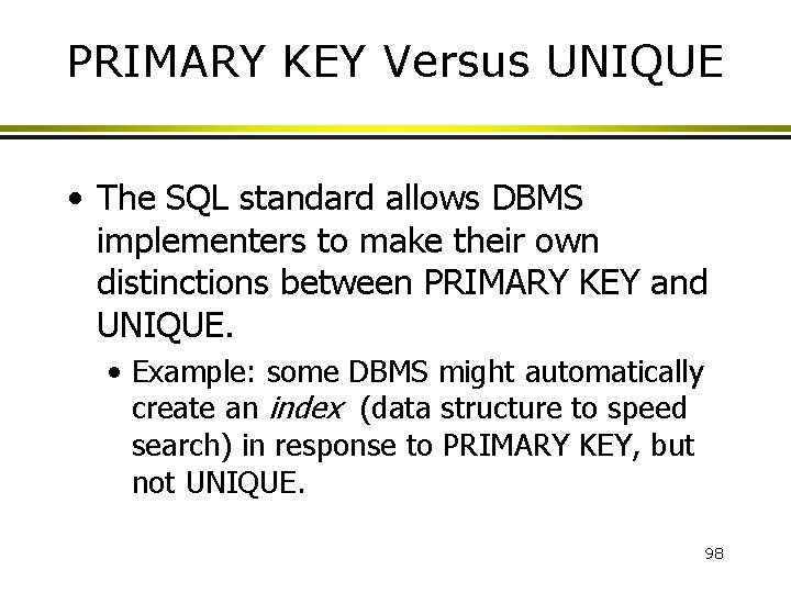
PRIMARY KEY Versus UNIQUE • The SQL standard allows DBMS implementers to make their own distinctions between PRIMARY KEY and UNIQUE. • Example: some DBMS might automatically create an index (data structure to speed search) in response to PRIMARY KEY, but not UNIQUE. 98

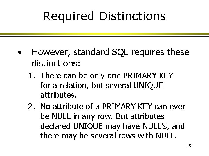
Required Distinctions • However, standard SQL requires these distinctions: 1. There can be only one PRIMARY KEY for a relation, but several UNIQUE attributes. 2. No attribute of a PRIMARY KEY can ever be NULL in any row. But attributes declared UNIQUE may have NULL’s, and there may be several rows with NULL. 99

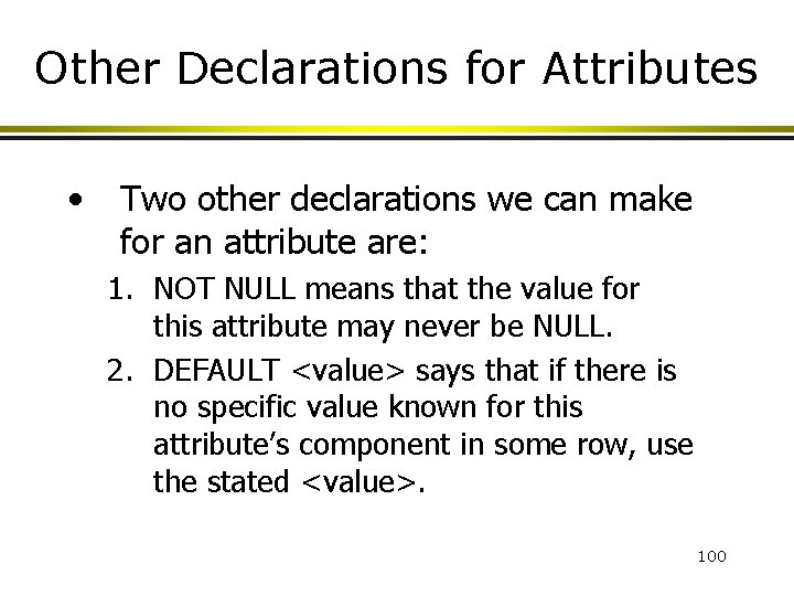
Other Declarations for Attributes • Two other declarations we can make for an attribute are: 1. NOT NULL means that the value for this attribute may never be NULL. 2. DEFAULT <value> says that if there is no specific value known for this attribute’s component in some row, use the stated <value>. 100

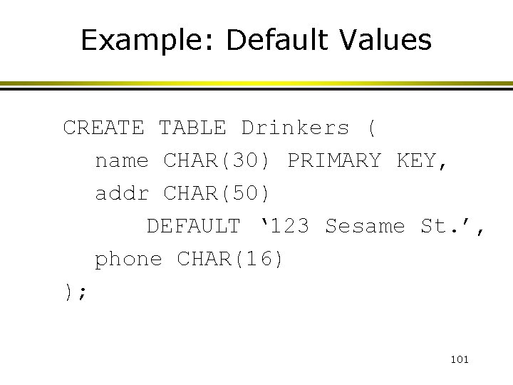
Example: Default Values CREATE TABLE Drinkers ( name CHAR(30) PRIMARY KEY, addr CHAR(50) DEFAULT ‘ 123 Sesame St. ’, phone CHAR(16) ); 101

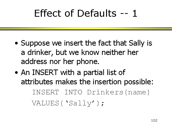
Effect of Defaults -- 1 • Suppose we insert the fact that Sally is a drinker, but we know neither address nor her phone. • An INSERT with a partial list of attributes makes the insertion possible: INSERT INTO Drinkers(name) VALUES(‘Sally’); 102

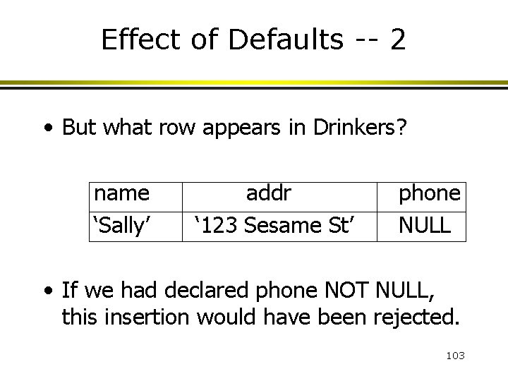
Effect of Defaults -- 2 • But what row appears in Drinkers? name ‘Sally’ addr ‘ 123 Sesame St’ phone NULL • If we had declared phone NOT NULL, this insertion would have been rejected. 103

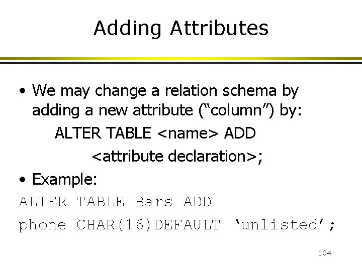
Adding Attributes • We may change a relation schema by adding a new attribute (“column”) by: ALTER TABLE <name> ADD <attribute declaration>; • Example: ALTER TABLE Bars ADD phone CHAR(16)DEFAULT ‘unlisted’; 104

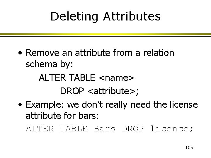
Deleting Attributes • Remove an attribute from a relation schema by: ALTER TABLE <name> DROP <attribute>; • Example: we don’t really need the license attribute for bars: ALTER TABLE Bars DROP license; 105

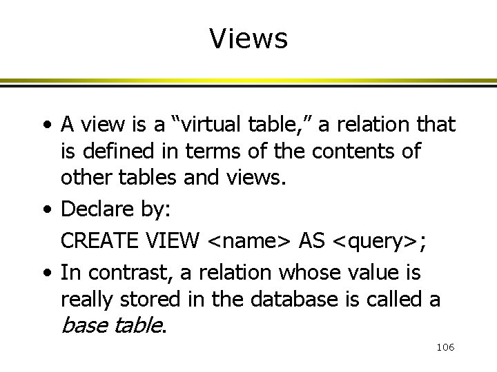
Views • A view is a “virtual table, ” a relation that is defined in terms of the contents of other tables and views. • Declare by: CREATE VIEW <name> AS <query>; • In contrast, a relation whose value is really stored in the database is called a base table. 106

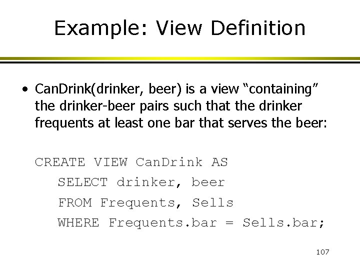
Example: View Definition • Can. Drink(drinker, beer) is a view “containing” the drinker-beer pairs such that the drinker frequents at least one bar that serves the beer: CREATE VIEW Can. Drink AS SELECT drinker, beer FROM Frequents, Sells WHERE Frequents. bar = Sells. bar; 107

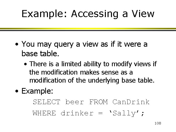
Example: Accessing a View • You may query a view as if it were a base table. • There is a limited ability to modify views if the modification makes sense as a modification of the underlying base table. • Example: SELECT beer FROM Can. Drink WHERE drinker = ‘Sally’; 108

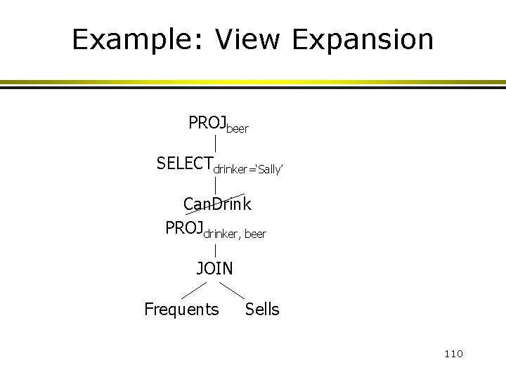
What Happens When a View Is Used? • The DBMS starts by interpreting the query as if the view were a base table. • Typical DBMS turns the query into something like relational algebra. • The queries defining any views used by the query are also replaced by their algebraic equivalents, and “spliced into” the expression tree for the query. 109

Example: View Expansion PROJbeer SELECTdrinker=‘Sally’ Can. Drink PROJdrinker, beer JOIN Frequents Sells 110

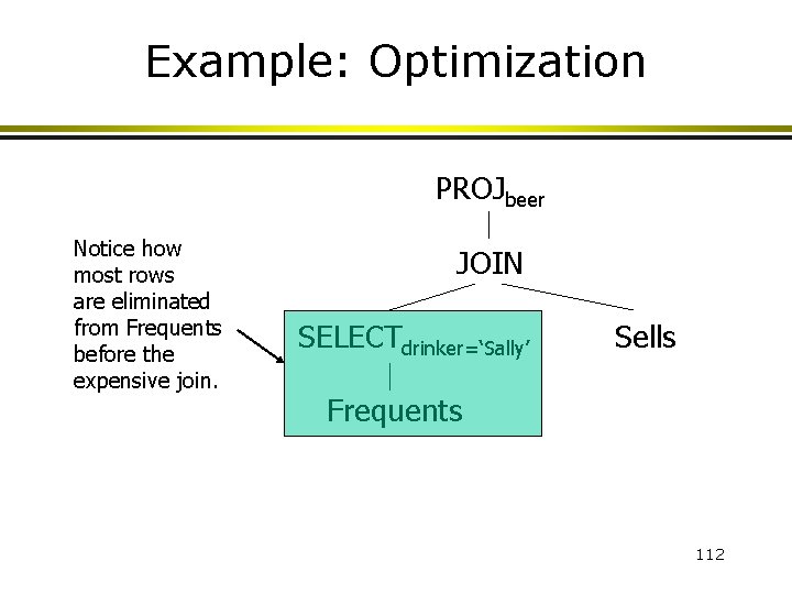
DMBS Optimization • • It is interesting to observe that the typical DBMS will then “optimize” the query by transforming the algebraic expression to one that can be executed faster. Key optimizations: 1. Push selections down the tree. 2. Eliminate unnecessary projections. 111

Example: Optimization PROJbeer Notice how most rows are eliminated from Frequents before the expensive join. JOIN SELECTdrinker=‘Sally’ Sells Frequents 112

More SQL? Foreign Keys Local and Global Constraints 113

Constraints • A constraint is a relationship among data elements that the DBMS is required to enforce. • Example: key constraints. 114

Kinds of Constraints • Keys. • Foreign-key, or referential-integrity. • Value-based constraints. • Constrain values of a particular attribute. • Row-based constraints. • Relationship among components. • Assertions: any SQL boolean expression. 115

Foreign Keys • Consider Relation Sells(bar, beer, price). • We might expect that a beer value is a real beer --- something appearing in Beers. name. • A constraint that requires a beer in Sells to be a beer in Beers is called a foreign key constraint. 116

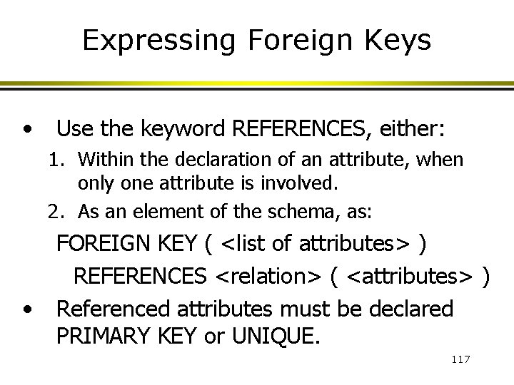
Expressing Foreign Keys • Use the keyword REFERENCES, either: 1. Within the declaration of an attribute, when only one attribute is involved. 2. As an element of the schema, as: • FOREIGN KEY ( <list of attributes> ) REFERENCES <relation> ( <attributes> ) Referenced attributes must be declared PRIMARY KEY or UNIQUE. 117

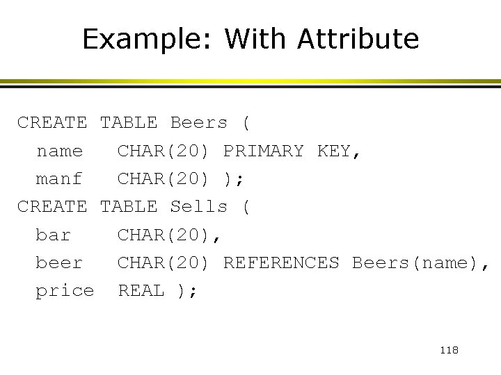
Example: With Attribute CREATE TABLE Beers ( name CHAR(20) PRIMARY KEY, manf CHAR(20) ); CREATE TABLE Sells ( bar CHAR(20), beer CHAR(20) REFERENCES Beers(name), price REAL ); 118

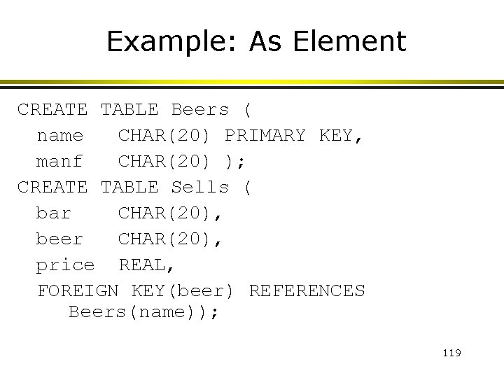
Example: As Element CREATE TABLE Beers ( name CHAR(20) PRIMARY KEY, manf CHAR(20) ); CREATE TABLE Sells ( bar CHAR(20), beer CHAR(20), price REAL, FOREIGN KEY(beer) REFERENCES Beers(name)); 119

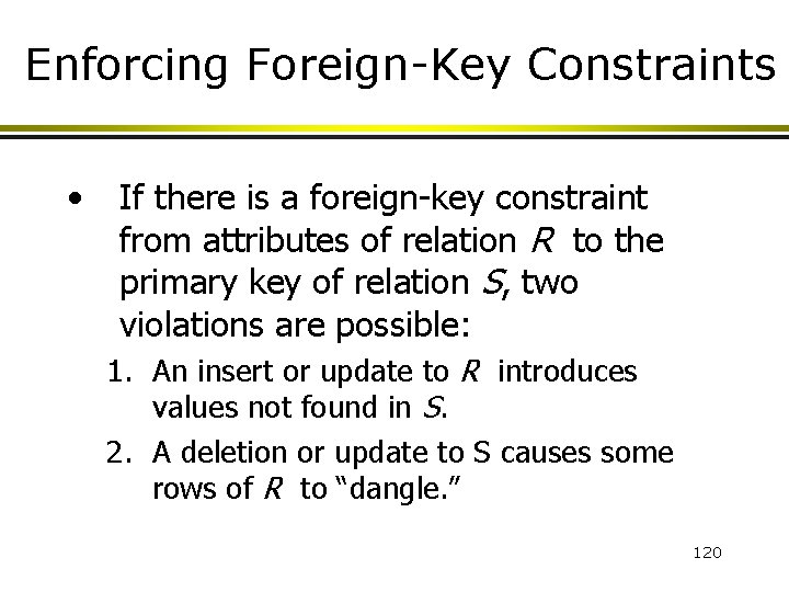
Enforcing Foreign-Key Constraints • If there is a foreign-key constraint from attributes of relation R to the primary key of relation S, two violations are possible: 1. An insert or update to R introduces values not found in S. 2. A deletion or update to S causes some rows of R to “dangle. ” 120

Actions Taken -- 1 • Suppose R = Sells, S = Beers. • An insert or update to Sells that introduces a nonexistent beer must be rejected. • A deletion or update to Beers that removes a beer value found in some rows of Sells can be handled in three ways. 121

Actions Taken -- 2 • The three possible ways to handle beers that suddenly cease to exist are: 1. Default : Reject the modification. 2. Cascade : Make the same changes in Sells. w Deleted beer: delete Sells row. w Updated beer: change value in Sells. 3. Set NULL : Change the beer to NULL. 122

Example: Cascade • Suppose we delete the Bud row from Beers. • Then delete all rows from Sells that have beer = ’Bud’. • Suppose we update the Bud row by changing ’Bud’ to ’Budweiser’. • Then change all Sells rows with beer = ’Bud’ so that beer = ’Budweiser’. 123

Example: Set NULL • Suppose we delete the Bud row from Beers. • Change all rows of Sells that have beer = ’Bud’ to have beer = NULL. • Suppose we update the Bud row by changing ’Bud’ to ’Budweiser’. • Same change. 124

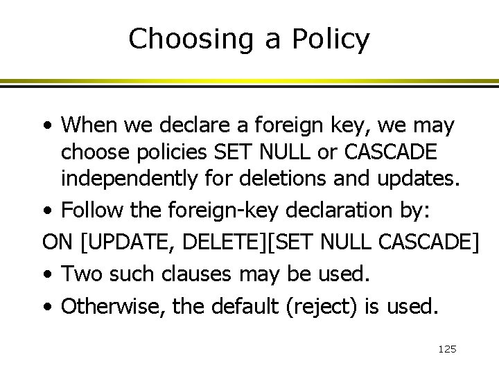
Choosing a Policy • When we declare a foreign key, we may choose policies SET NULL or CASCADE independently for deletions and updates. • Follow the foreign-key declaration by: ON [UPDATE, DELETE][SET NULL CASCADE] • Two such clauses may be used. • Otherwise, the default (reject) is used. 125

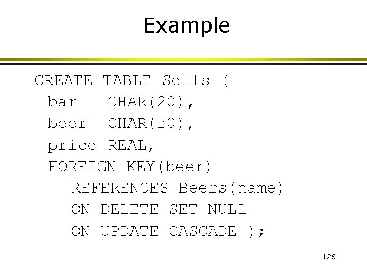
Example CREATE TABLE Sells ( bar CHAR(20), beer CHAR(20), price REAL, FOREIGN KEY(beer) REFERENCES Beers(name) ON DELETE SET NULL ON UPDATE CASCADE ); 126

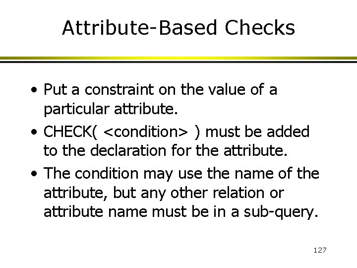
Attribute-Based Checks • Put a constraint on the value of a particular attribute. • CHECK( <condition> ) must be added to the declaration for the attribute. • The condition may use the name of the attribute, but any other relation or attribute name must be in a sub-query. 127

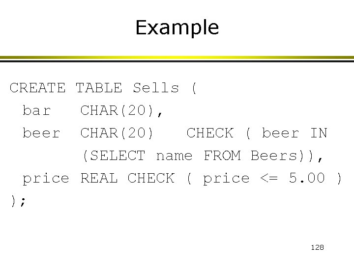
Example CREATE TABLE Sells ( bar CHAR(20), beer CHAR(20) CHECK ( beer IN (SELECT name FROM Beers)), price REAL CHECK ( price <= 5. 00 ) ); 128

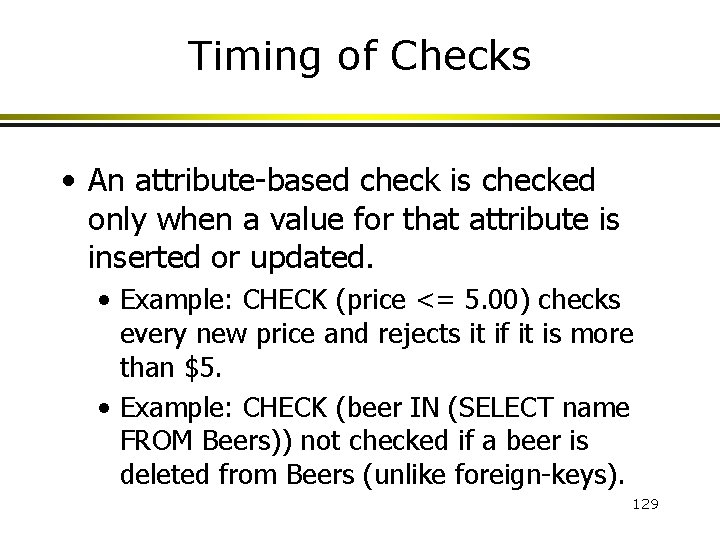
Timing of Checks • An attribute-based check is checked only when a value for that attribute is inserted or updated. • Example: CHECK (price <= 5. 00) checks every new price and rejects it if it is more than $5. • Example: CHECK (beer IN (SELECT name FROM Beers)) not checked if a beer is deleted from Beers (unlike foreign-keys). 129

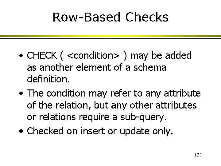
Row-Based Checks • CHECK ( <condition> ) may be added as another element of a schema definition. • The condition may refer to any attribute of the relation, but any other attributes or relations require a sub-query. • Checked on insert or update only. 130

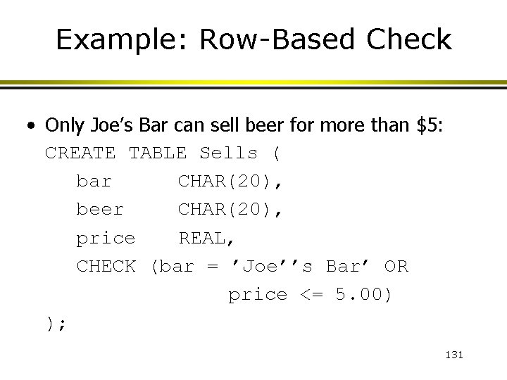
Example: Row-Based Check • Only Joe’s Bar can sell beer for more than $5: CREATE TABLE Sells ( bar CHAR(20), beer CHAR(20), price REAL, CHECK (bar = ’Joe’’s Bar’ OR price <= 5. 00) ); 131

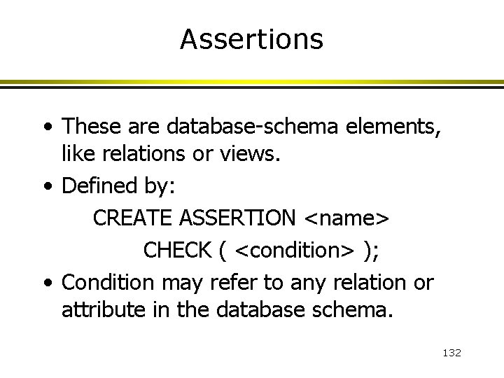
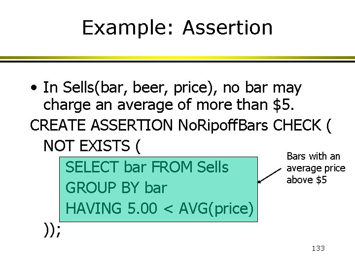
Assertions • These are database-schema elements, like relations or views. • Defined by: CREATE ASSERTION <name> CHECK ( <condition> ); • Condition may refer to any relation or attribute in the database schema. 132

Example: Assertion • In Sells(bar, beer, price), no bar may charge an average of more than $5. CREATE ASSERTION No. Ripoff. Bars CHECK ( NOT EXISTS ( Bars with an average price SELECT bar FROM Sells above $5 GROUP BY bar HAVING 5. 00 < AVG(price) )); 133

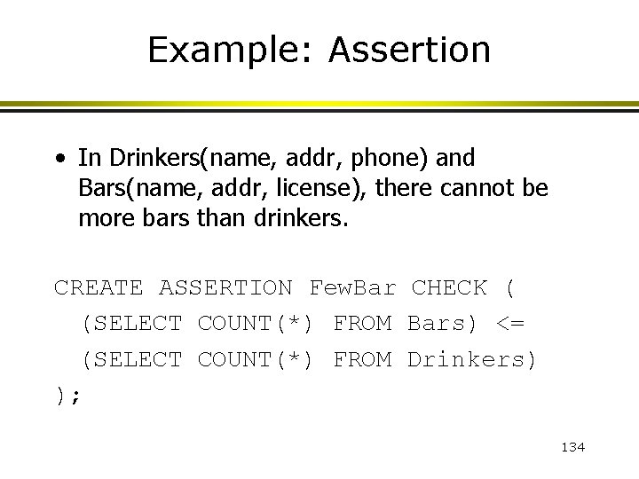
Example: Assertion • In Drinkers(name, addr, phone) and Bars(name, addr, license), there cannot be more bars than drinkers. CREATE ASSERTION Few. Bar CHECK ( (SELECT COUNT(*) FROM Bars) <= (SELECT COUNT(*) FROM Drinkers) ); 134

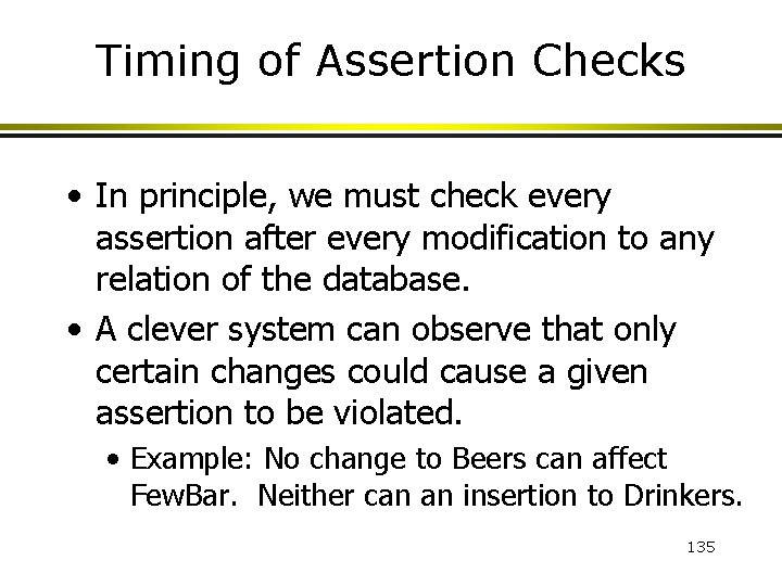
Timing of Assertion Checks • In principle, we must check every assertion after every modification to any relation of the database. • A clever system can observe that only certain changes could cause a given assertion to be violated. • Example: No change to Beers can affect Few. Bar. Neither can an insertion to Drinkers. 135

End of Lecture 136