Introduction to Sorting Methods Basics of Sorting Elementary

Introduction to Sorting Methods – Basics of Sorting – Elementary Sorting Algorithms • Selection sort • Insertion sort • Shellsort

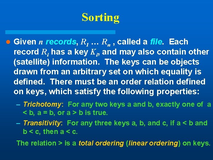
Sorting l Given n records, R 1 … Rn , called a file. Each record Ri has a key Ki, and may also contain other (satellite) information. The keys can be objects drawn from an arbitrary set on which equality is defined. There must be an order relation defined on keys, which satisfy the following properties: – Trichotomy: For any two keys a and b, exactly one of a < b, a = b, or a > b is true. – Transitivity: For any three keys a, b, and c, if a < b and b < c, then a < c. The relation > is a total ordering (linear ordering) on keys.

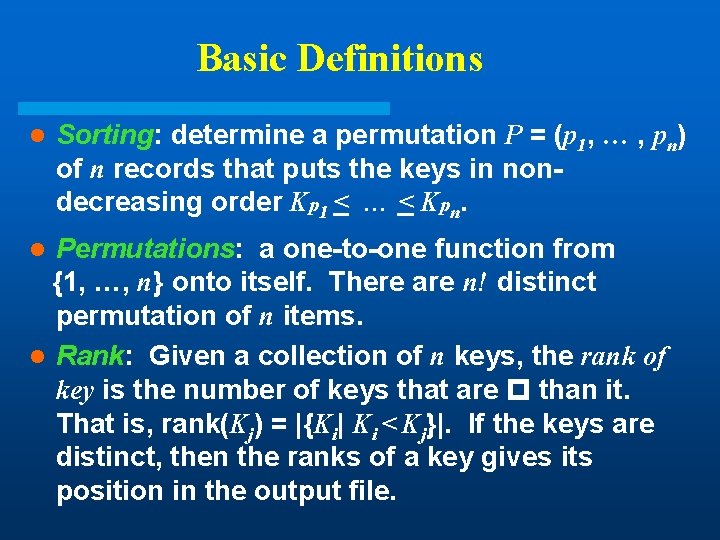
Basic Definitions l Sorting: determine a permutation P = (p 1, … , pn) of n records that puts the keys in nondecreasing order Kp 1 < … < Kpn. Permutations: a one-to-one function from {1, …, n} onto itself. There are n! distinct permutation of n items. l Rank: Given a collection of n keys, the rank of key is the number of keys that are than it. That is, rank(Kj) = |{Ki| Ki < Kj}|. If the keys are distinct, then the ranks of a key gives its position in the output file. l

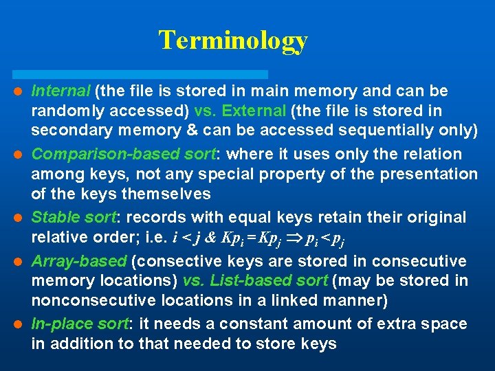
Terminology l l l Internal (the file is stored in main memory and can be randomly accessed) vs. External (the file is stored in secondary memory & can be accessed sequentially only) Comparison-based sort: where it uses only the relation among keys, not any special property of the presentation of the keys themselves Stable sort: records with equal keys retain their original relative order; i. e. i < j & Kpi = Kpj pi < pj Array-based (consective keys are stored in consecutive memory locations) vs. List-based sort (may be stored in nonconsecutive locations in a linked manner) In-place sort: it needs a constant amount of extra space in addition to that needed to store keys

Elementary Sorting Methods l Easier to understand the basic mechanisms of sorting l Maybe more suitable for small files l Good for well-structured files that are relatively easy to sort, such as those almost sorted l Can be used to improve efficiency of more powerful methods

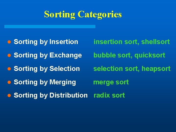
Sorting Categories l Sorting by Insertion insertion sort, shellsort l Sorting by Exchange bubble sort, quicksort l Sorting by Selection sort, heapsort l Sorting by Merging merge sort l Sorting by Distribution radix sort

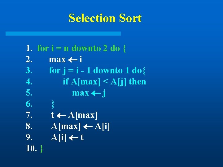
Selection Sort 1. for i = n downto 2 do { 2. max i 3. for j = i - 1 downto 1 do{ 4. if A[max] < A[j] then 5. max j 6. } 7. t A[max] 8. A[max] A[i] 9. A[i] t 10. }

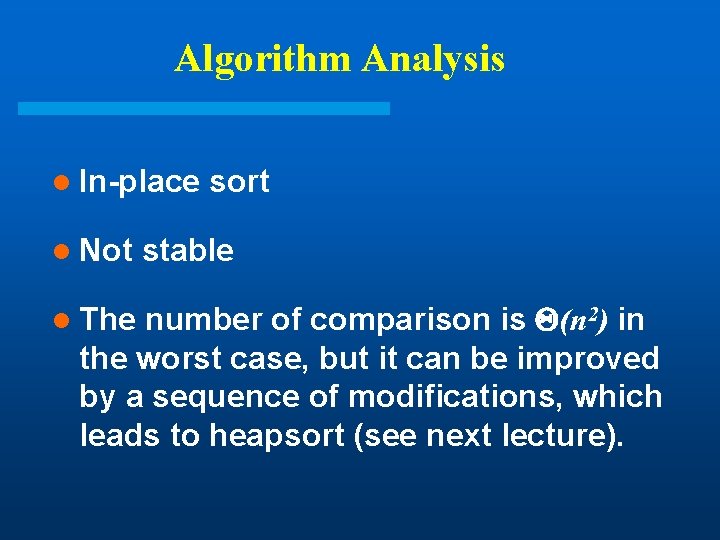
Algorithm Analysis l In-place l Not sort stable number of comparison is (n 2) in the worst case, but it can be improved by a sequence of modifications, which leads to heapsort (see next lecture). l The

Insertion Sort 1. for j = 2 to n do { 2. key A[j] 3. i j-1 4. while i > 0 and key < A[i] { 5. A[i+1] A[i] 6. i i-1 7. } 8. A[i+1] key 9. }

Algorithm Analysis l In-place sort l Stable l If A is sorted: (n) comparisons l If A is reversed sorted: (n 2) comparisons l If A is randomly sorted: (n 2) comparisons

Worst Case Analysis l The maximum number of comparison while inserting A[i] is (i-1). So, the number of comparison is Cwc(n) i = 2 to n (i -1) j = 1 to n-1 j = n(n-1)/2 = (n 2)

Average Case Analysis l Consider when we try to insert the key A[i]. There are i places where it can end up after insertion. Assume all possibilities are equally likely with probability of 1/i. Then, the average number of comparisons to insert A[i] is j = 1 to i-1 [ 1/i * j ] + 1/i * (i - 1) = (i+1)/2 - 1/i l Summing over insertion of all keys, we get Cavg(n) = i = 2 to n [(i+1)/2 - 1/i] = n 2/4 + 3 n/4 - 1 - ln n = (n 2 ) l Therefore, Tavg(n) = (n 2 )

Analysis of Inversions in Permutation l Worst Case: n(n-1)/2 inversions l Average Case: – Consider each permutation and its transpose permutation T. Given any , T is unique and T – Consider the pair (i, j) with i < j, there are n(n-1)/2 pairs. – (i, j) is an inversion of if and only if (n-j, n-i) is not an inversion of T. This implies that the pair ( , T) together have n(n-1)/2 inversions. The average number of inversions is n(n-1)/4.

Theorem l Any algorithm that sorts by comparison of keys and removes at most one inversion after each comparison must do at least n(n-1)/2 comparisons in the worst case and at least n(n-1)/4 comparisons on the average. If we want to do better than (n 2) , we have to remove more than a constant number of inversions with each comparison.

Insertion Sort to Shellsort is a simple extension of insertion sort. It gains speed by allowing exchanges with elements that are far apart. l The idea is that rearrangement of the file by taking every hth element (starting anywhere) yield a sorted file. Such a file is “h-sorted”. A “h-sorted” file is h independent sorted files, interleaved together. l By h-sorting for some large values of “increment” h, we can move records far apart and thus make it easier for h-sort for smaller values of h. Using such a procedure for any sequence of values of h which ends in 1 will produce a sorted file. l

Shellsort l A family of algorithms, characterized by the sequence {hk} of increments that are used in sorting. l By interleaving, we can fix multiple inversions with each comparisons, so that later passes see files that are “nearly sorted”. This implies that eithere are many keys not too far from their final position, or only a small number of keys are far off.

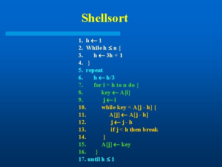
Shellsort 1. h 1 2. While h n { 3. h 3 h + 1 4. } 5. repeat 6. h h/3 7. for i = h to n do { 8. key A[i] 9. j i 10. while key < A[j - h] { 11. A[j] A[j - h] 12. j j-h 13. if j < h then break 14. } 15. A[j] key 16. } 17. until h 1

Algorithm Analysis l In-place l Not sort stable l The exact behavior of the algorithm depends on the sequence of increments -- difficult & complex to analyze the algorithm. l For hk = 2 k - 1, T(n) = (n 3/2 )

Heapsort l Heapsort – Data Structure – Maintain the Heap Property – Build a Heap – Heapsort Algorithm – Priority Queue

Heap Data Structure in (n) time l Extract maximum element in (lg n) time l Leads to (n lg n) sorting algorithm: l Construct – Build heap – Repeatedly extract largest remaining element (constructing sorted list from back to front) l Heaps useful for other purposes too

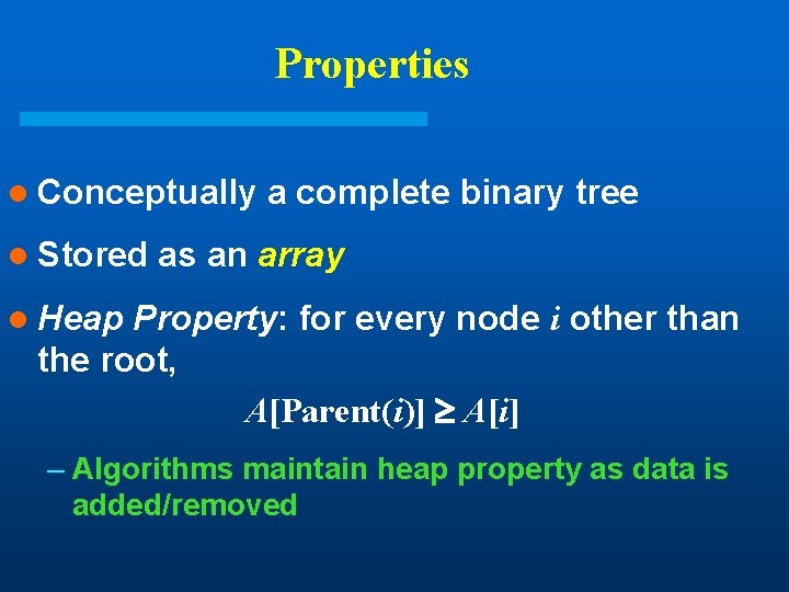
Properties l Conceptually l Stored a complete binary tree as an array l Heap Property: for every node i other than the root, A[Parent(i)] A[i] – Algorithms maintain heap property as data is added/removed

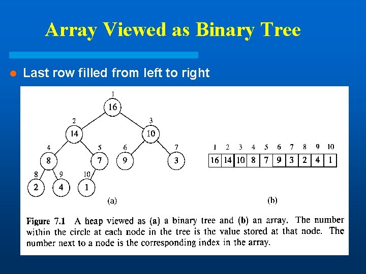
Array Viewed as Binary Tree l Last row filled from left to right

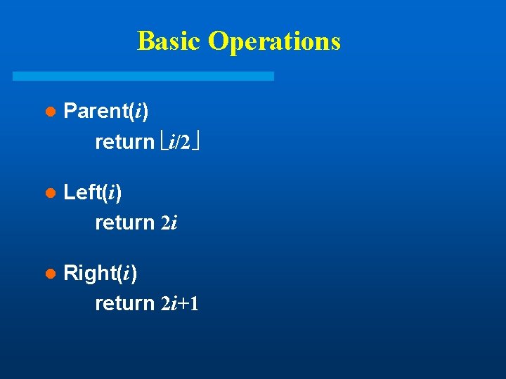
Basic Operations l Parent(i) return i/2 l Left(i) return 2 i l Right(i) return 2 i+1

Height l Height of a node in a tree: the number of edges on the longest simple downward path from the node to a leaf l Height of a tree: the height of the root l Height of the tree for a heap: (lg n) – Basic operations on a heap run in O(lg n) time

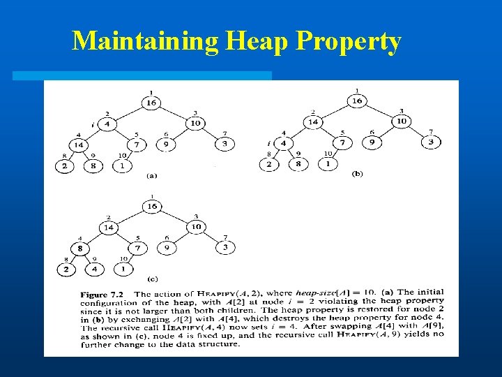
Maintaining Heap Property

Heapify (A, i) 1. l left(i) 2. r right(i) 3. if l heap-size[A] and A[l] > A[i] 4. then largest l 5. else largest i 6. if r heap-size[A] and A[r] > A[largest] 7. then largest r 8. if largest i 9. then exchange A[i] A[largest] 10. Heapify(A, largest)

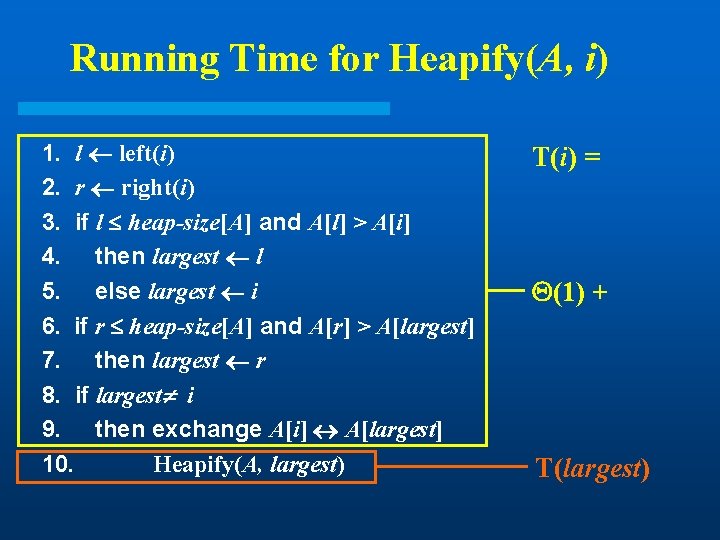
Running Time for Heapify(A, i) 1. l left(i) 2. r right(i) 3. if l heap-size[A] and A[l] > A[i] 4. then largest l 5. else largest i 6. if r heap-size[A] and A[r] > A[largest] 7. then largest r 8. if largest i 9. then exchange A[i] A[largest] 10. Heapify(A, largest) T(i) = (1) + T(largest)

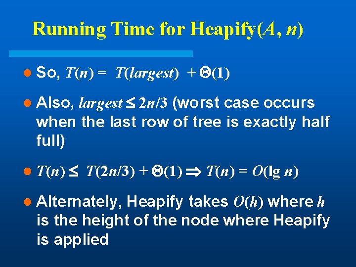
Running Time for Heapify(A, n) l So, T(n) = T(largest) + (1) largest 2 n/3 (worst case occurs when the last row of tree is exactly half full) l Also, l T(n) T(2 n/3) + (1) T(n) = O(lg n) l Alternately, Heapify takes O(h) where h is the height of the node where Heapify is applied

Build-Heap(A) 1. heap-size[A] length[A] 2. for i length[A]/2 downto 1 3. do Heapify(A, i)

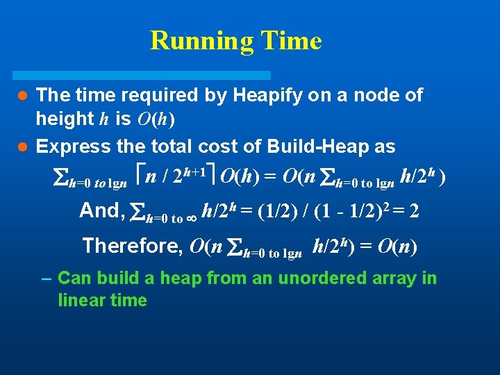
Running Time The time required by Heapify on a node of height h is O(h) l Express the total cost of Build-Heap as l h=0 to lgn n / 2 h+1 O(h) = O(n h=0 to lgn h/2 h ) And, h=0 to h/2 h = (1/2) / (1 - 1/2)2 = 2 Therefore, O(n h=0 to lgn h/2 h) = O(n) – Can build a heap from an unordered array in linear time

Heapsort (A) 1. Build-Heap(A) 2. for i length[A] downto 2 3. do exchange A[1] A[i] 4. heap-size[A] - 1 5. Heapify(A, 1)

Algorithm Analysis l In-place l Not Stable l Build-Heap takes O(n) and each of the n-1 calls to Heapify takes time O(lg n). l Therefore, T(n) = O(n lg n)

Priority Queues l A data structure for maintaining a set S of elements, each with an associated value called a key. l Applications: scheduling jobs on a shared computer, prioritizing events to be processed based on their predicted time of occurrence. l Heap can be used to implement a priority queue.

Basic Operations l Insert(S, x) - inserts the element x into the set S, i. e. S S {x} l Maximum(S) - returns the element of S with the largest key l Extract-Max(S) - removes and returns the element of S with the largest key

Heap-Extract-Max(A) 1. 2. 3. 4. 5. 6. 7. if heap-size[A] < 1 then error “heap underflow” max A[1] A[heap-size[A]] heap-size[A] - 1 Heapify(A, 1) return max

Heap-Insert(A, key) 1. 2. 3. 4. 5. 6. heap-size[A] + 1 i heap-size[A] while i > 1 and A[Parent(i)] < key do A[i] A[Parent(i)] i Parent(i) A[i] key

Running Time l Running time of Heap-Extract-Max is O(lg n). – Performs only a constant amount of work on top of Heapify, which takes O(lg n) time l Running time of Heap-Insert is O(lg n). – The path traced from the new leaf to the root has length O(lg n).

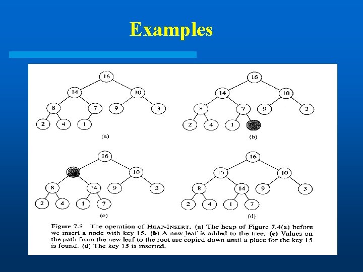
Examples

Quick. Sort l Divide: A[p…r] is partitioned (rearranged) into two nonempty subarrays A[p…q] and A[q+1…r] s. t. each element of A[p…q] is less than or equal to each element of A[q+1…r]. Index q is computed here. l Conquer: two subarrays are sorted by recursive calls to quicksort. l Combine: no work needed since the subarrays are sorted in place already.

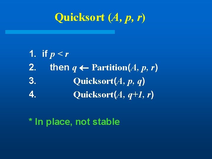
Quicksort (A, p, r) 1. if p < r 2. then q Partition(A, p, r) 3. Quicksort(A, p, q) 4. Quicksort(A, q+1, r) * In place, not stable

Partition(A, p, r) 1. x A[p] 2. i p - 1 3. j r + 1 4. while TRUE 5. do repeat j j - 1 6. until A[j] x 7. repeat i i + 1 8. until A[i] x 9. if i < j 10. then exchange A[i] A[j] 11. else return j

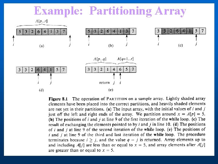
Example: Partitioning Array

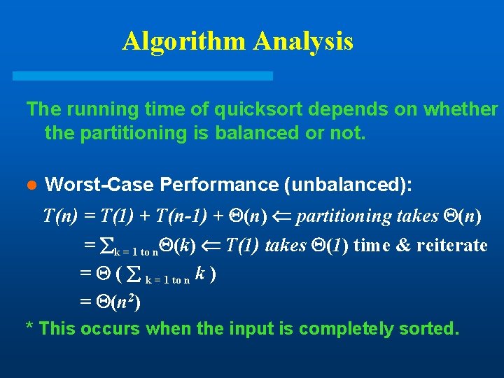
Algorithm Analysis The running time of quicksort depends on whether the partitioning is balanced or not. l Worst-Case Performance (unbalanced): T(n) = T(1) + T(n-1) + (n) partitioning takes (n) = k = 1 to n (k) T(1) takes (1) time & reiterate = ( k = 1 to n k ) = (n 2) * This occurs when the input is completely sorted.

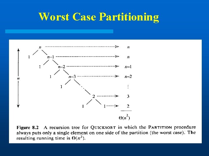
Worst Case Partitioning

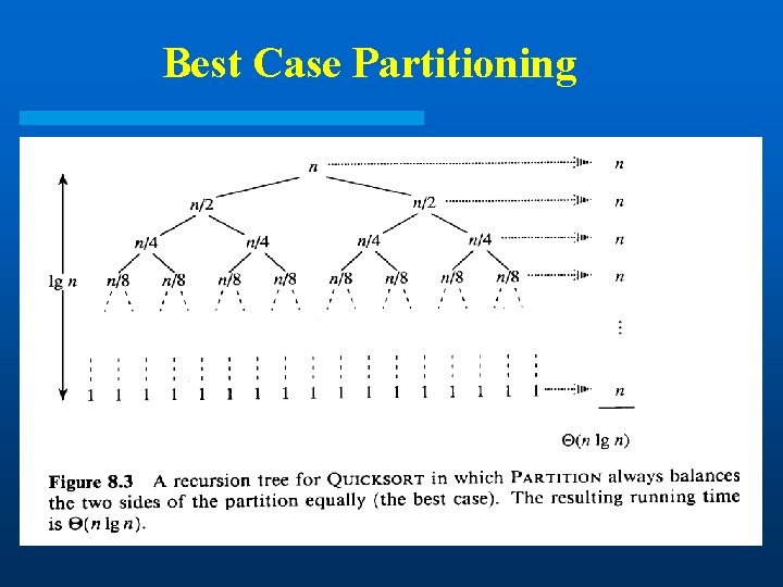
Best Case Partitioning

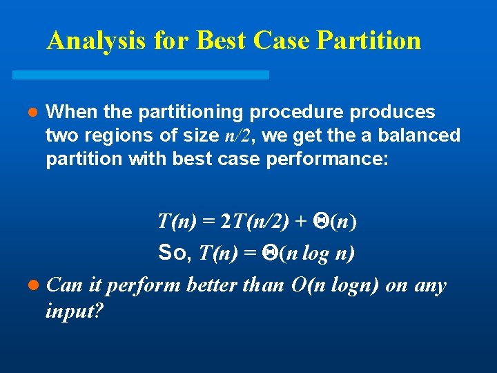
Analysis for Best Case Partition l When the partitioning procedure produces two regions of size n/2, we get the a balanced partition with best case performance: T(n) = 2 T(n/2) + (n) So, T(n) = (n log n) l Can it perform better than O(n logn) on any input?

Average-Case Behavior l For example, when the partitioning algorithm always produces a 7 -to-3 proportional split: T(n) = T(7 n/10) + T(3 n/10) + n Solve the recurrence by visualizing recursion tree, each level has a cost of n with the height of lg n. So, we get T(n) = (n log n) when the split has constant proportionality. l For a split of proportionality , where 0 1/2, the minimum depth of the tree is - lg n / lg and the maximum depth is - lg n / lg (1 - ).

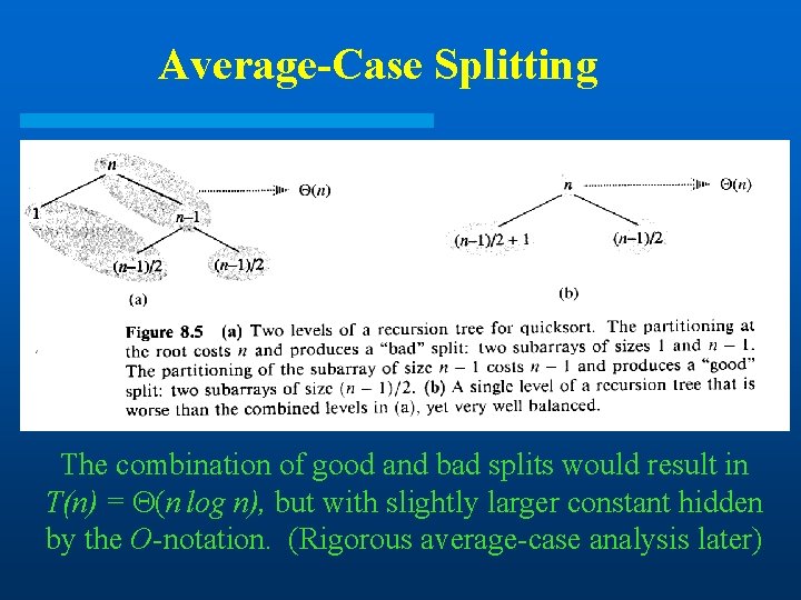
Average-Case Splitting The combination of good and bad splits would result in T(n) = (n log n), but with slightly larger constant hidden by the O-notation. (Rigorous average-case analysis later)

Randomized Quicksort l An algorithm is randomized if its behavior is determined not only by the input but also by values produced by a random-number generator. No particular input elicits worst-case behavior. Two possible versions of quicksort: – Impose a distribution on input to ensure that every permutation is equally likely. This does not improve the worst-case running time, but makes run time independent of input ordering. – Exchange A[p] with an element chosen at random from A[p…r] in Partition. This ensures that the pivot element is equally likely to be any of input elements.

Randomized-Partition(A, p, r) 1. i Random (p, r) 2. exchange A[p] A[i] 3. return Partition(A, p, r)

Randomized-Quicksort (A, p, r) 1. if p < r 2. then q Randomized-Partition(A, p, r) 3. Randomized-Quicksort(A, p, q) 4. Randomized-Quicksort(A, q+1, r)

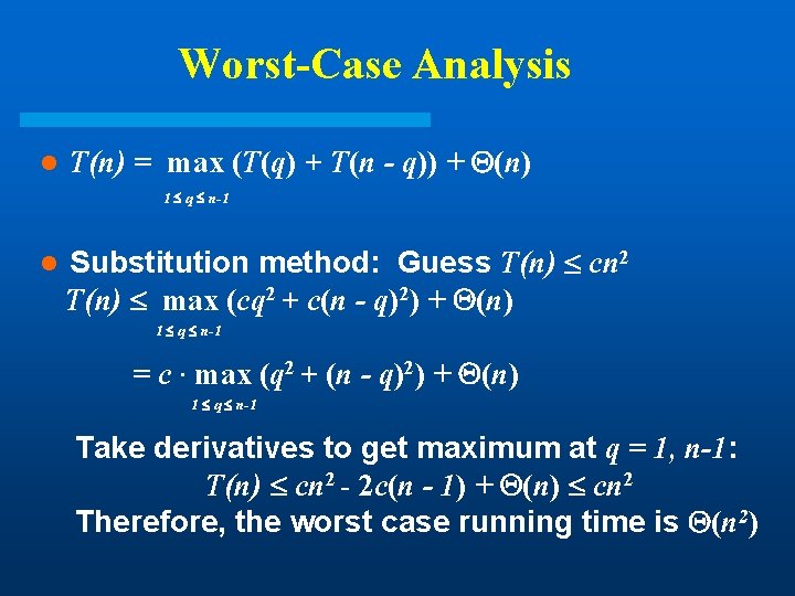
Worst-Case Analysis l T(n) = max (T(q) + T(n - q)) + (n) 1 q n-1 l Substitution method: Guess T(n) cn 2 T(n) max (cq 2 + c(n - q)2) + (n) 1 q n-1 = c · max (q 2 + (n - q)2) + (n) 1 q n-1 Take derivatives to get maximum at q = 1, n-1: T(n) cn 2 - 2 c(n - 1) + (n) cn 2 Therefore, the worst case running time is (n 2)

Average-Case Analysis l Partitioning depends only on the rank of x =A[p]. l When rank(x) = 1, index i stops at i = p and j stops j = p. q = p is returned. So, the probability of the low side has one element is 1/n. l When rank(x) 2, there is at least one element smaller than x =A[p]. When the “Partition” terminates, each of the rank(x)-1 elements in the low side of the partition is strictly less than x. For each i = 1, … , n-1, the probability is 1/n that the low side has i elements.

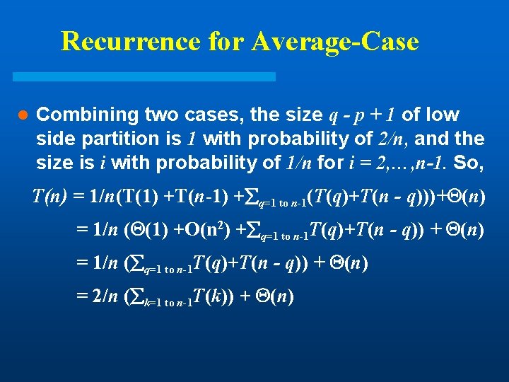
Recurrence for Average-Case l Combining two cases, the size q - p + 1 of low side partition is 1 with probability of 2/n, and the size is i with probability of 1/n for i = 2, …, n-1. So, T(n) = 1/n(T(1) +T(n-1) + q=1 to n-1(T(q)+T(n - q)))+ (n) = 1/n ( (1) +O(n 2) + q=1 to n-1 T(q)+T(n - q)) + (n) = 1/n ( q=1 to n-1 T(q)+T(n - q)) + (n) = 2/n ( k=1 to n-1 T(k)) + (n)

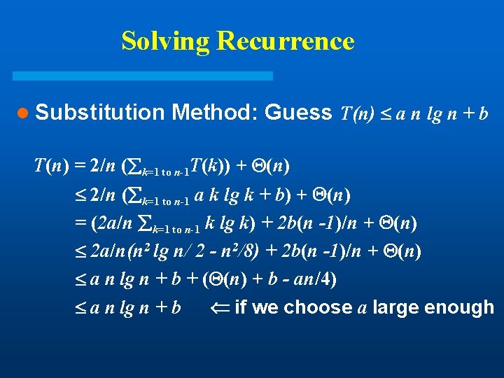
Solving Recurrence l Substitution Method: Guess T(n) a n lg n + b T(n) = 2/n ( k=1 to n-1 T(k)) + (n) 2/n ( k=1 to n-1 a k lg k + b) + (n) = (2 a/n k=1 to n-1 k lg k) + 2 b(n -1)/n + (n) 2 a/n(n 2 lg n/ 2 - n 2/8) + 2 b(n -1)/n + (n) a n lg n + b + ( (n) + b - an/4) a n lg n + b if we choose a large enough

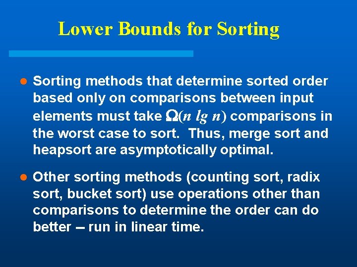
Lower Bounds for Sorting l Sorting methods that determine sorted order based only on comparisons between input elements must take (n lg n) comparisons in the worst case to sort. Thus, merge sort and heapsort are asymptotically optimal. l Other sorting methods (counting sort, radix sort, bucket sort) use operations other than comparisons to determine the order can do better -- run in linear time.

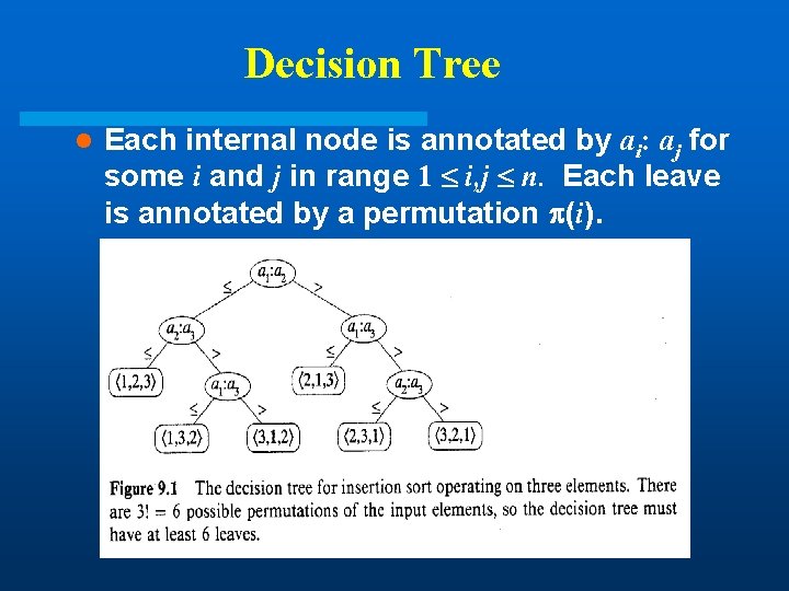
Decision Tree l Each internal node is annotated by ai: aj for some i and j in range 1 i, j n. Each leave is annotated by a permutation (i).

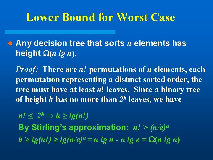
Lower Bound for Worst Case l Any decision tree that sorts n elements has height (n lg n). Proof: There are n! permutations of n elements, each permutation representing a distinct sorted order, the tree must have at least n! leaves. Since a binary tree of height h has no more than 2 h leaves, we have n! 2 h h lg(n!) By Stirling’s approximation: n! > (n/e)n h lg(n!) lg(n/e)n = n lg n - n lg e = (n lg n)

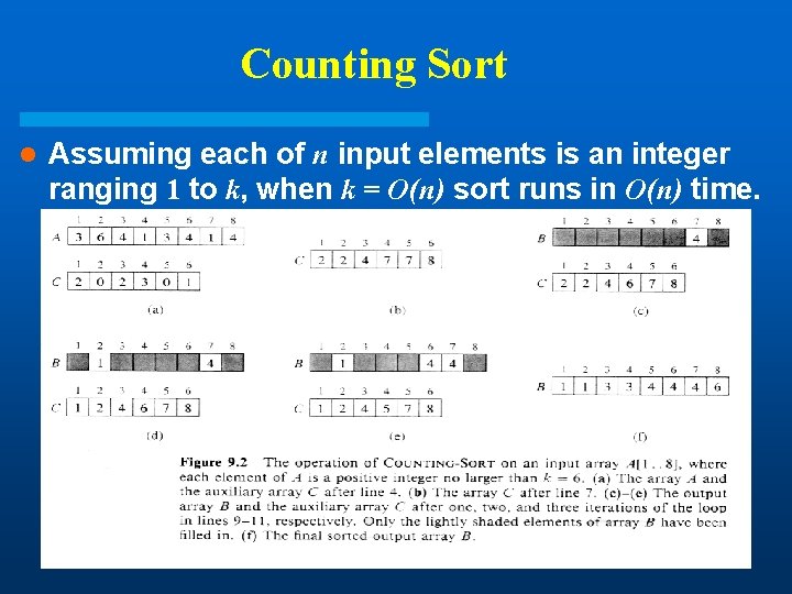
Counting Sort l Assuming each of n input elements is an integer ranging 1 to k, when k = O(n) sort runs in O(n) time.

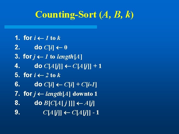
Counting-Sort (A, B, k) 1. 2. 3. 4. 5. 6. 7. 8. 9. for i 1 to k do C[i] 0 for j 1 to length[A] do C[A[j]] + 1 for i 2 to k do C[i] + C[i-1] for j length[A] downto 1 do B[C[A[ j ]]] A[j] C[A[j]] - 1

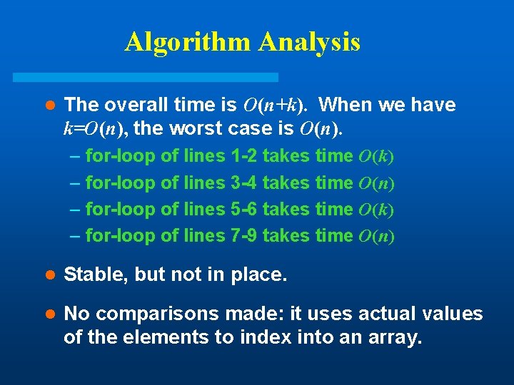
Algorithm Analysis l The overall time is O(n+k). When we have k=O(n), the worst case is O(n). – for-loop of lines 1 -2 takes time O(k) – for-loop of lines 3 -4 takes time O(n) – for-loop of lines 5 -6 takes time O(k) – for-loop of lines 7 -9 takes time O(n) l Stable, but not in place. l No comparisons made: it uses actual values of the elements to index into an array.

Radix Sort l It was used by the card-sorting machines to read the punch cards. l The key is sort the “least significant digit” first and the remaining digits in sequential order. The sorting method used to sort each digit must be “stable”. – If we start with the “most significant digit”, we’ll need extra storage.

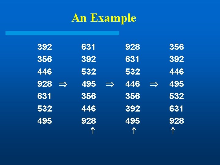
An Example 392 356 446 928 631 532 495 631 392 532 495 356 446 928 631 532 446 356 392 495 356 392 446 495 532 631 928

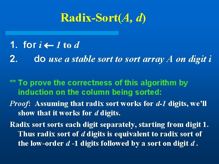
Radix-Sort(A, d) 1. for i 1 to d 2. do use a stable sort to sort array A on digit i ** To prove the correctness of this algorithm by induction on the column being sorted: Proof: Assuming that radix sort works for d-1 digits, we’ll show that it works for d digits. Radix sorts each digit separately, starting from digit 1. Thus radix sort of d digits is equivalent to radix sort of the low-order d -1 digits followed by a sort on digit d.

Correctness of Radix Sort By our induction hypothesis, the sort of the low-order d-1 digits works, so just before the sort on digit d , the elements are in order according to their low-order d-1 digits. The sort on digit d will order the elements by their dth digit. Consider two elements, a and b, with digits ad and bd: l If ad < bd , the sort will put a before b, since a < b regardless of the low-order digits. l If ad > bd , the sort will put a after b, since a > b regardless of the low-order digits. l If ad = bd , the sort will leave a and b in the same order, since the sort is stable. But that order is already correct, since the correct order of is determined by the low-order digits when their dth digits are equal.

Algorithm Analysis l Each pass over n d-digit numbers then takes time (n+k). l There are d passes, so the total time for radix sort is (d n+ d k). l When d is a constant and k = O(n), radix sort runs in linear time. l Radix sort, if uses counting sort as the intermediate stable sort, does not sort in place. – If primary memory storage is an issue, quicksort or other sorting methods may be preferable.

Bucket Sort l Counting sort and radix sort are good for integers. For floating point numbers, try bucket sort or other comparison-based methods. l Assume that input is generated by a random process that distributes the elements uniformly over interval [0, 1). (Other ranges can be scaled accordingly. ) l The basic idea is to divide the interval into n equalsized subintervals, or “buckets”, then insert the n input numbers into the buckets. The elements in each bucket are then sorted; lists from all buckets are concatenated in sequential order to generate output.

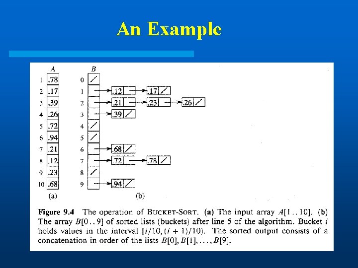
An Example

Bucket-Sort (A) 1. 2. 3. 4. 5. 6. n length[A] for i 1 to n do insert A[i] into list B[ n. A[i] ] for i 0 to n-1 do sort list B[i] with insertion sort Concatenate the lists B[i]s together in order

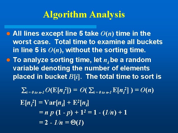
Algorithm Analysis All lines except line 5 take O(n) time in the worst case. Total time to examine all buckets in line 5 is O(n), without the sorting time. l To analyze sorting time, let ni be a random variable denoting the number of elements placed in bucket B[i]. The total time to sort is l i = 0 to n-1 O(E[ni 2]) = O( i = 0 to n-1 E[ni 2] ) = O(n) E[ni 2] = Var[ni] + E 2[ni] = n p (1 - p) + 12 = 1 - (1/n) + 1 = 2 - 1/n = (1)

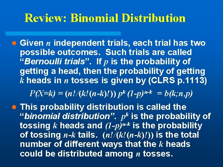
Review: Binomial Distribution l Given n independent trials, each trial has two possible outcomes. Such trials are called “Bernoulli trials”. If p is the probability of getting a head, then the probability of getting k heads in n tosses is given by (CLRS p. 1113) P(X=k) = (n!/(k!(n-k)!)) pk (1 -p)n-k = b(k; n, p) l This probability distribution is called the “binomial distribution”. pk is the probability of tossing k heads and (1 -p)n-k is the probability of tossing n-k tails. (n!/(k!(n-k)!)) is the total number of different ways that the k heads could be distributed among n tosses.

Review: Binomial Distribution See p. 1113 -1116 for the derivations. l E[x] =np l Var[x] l E[X 2] = E[X 2] - E 2[X] = n p (1 -p) = Var[X] + E 2[X] = n p (1 -p) + (n p)2 = 1(1 -p) + 12

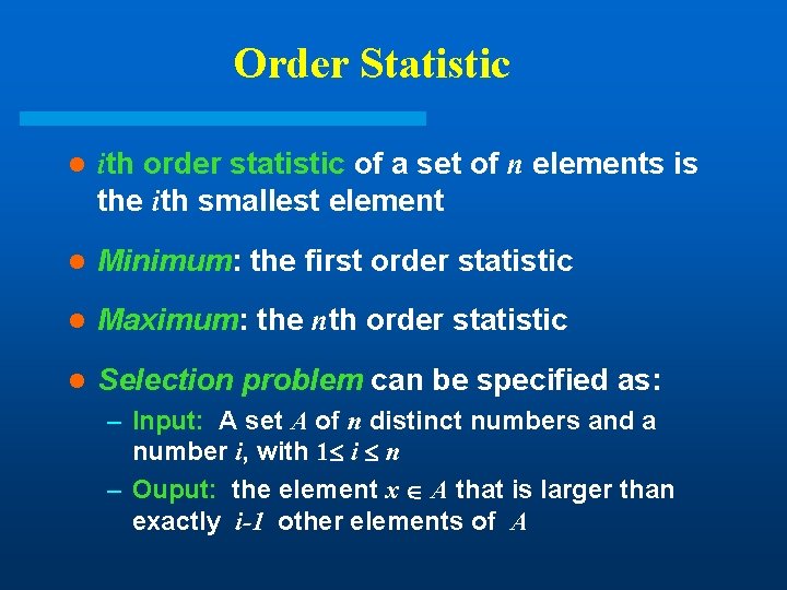
Order Statistic l ith order statistic of a set of n elements is the ith smallest element l Minimum: the first order statistic l Maximum: the nth order statistic l Selection problem can be specified as: – Input: A set A of n distinct numbers and a number i, with 1 i n – Ouput: the element x A that is larger than exactly i-1 other elements of A

Minimum (A) 1. min A[1] 2. for i 2 to length[A] 3. do if min > A[i] 4. then min A[i] 5. return min

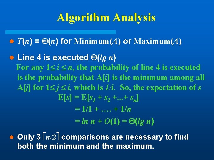
Algorithm Analysis l T(n) = (n) for Minimum(A) or Maximum(A) l Line 4 is executed (lg n) For any 1 i n, the probability of line 4 is executed is the probability that A[i] is the minimum among all A[j] for 1 j i, which is 1/i. So, the expectation of s E[s] = E[s 1 + s 2 +. . . + sn] = 1/1 + …. + 1/n = ln n + O(1) = (lg n) l Only 3 n/2 comparisons are necessary to find both the minimum and the maximum.

Randomized-Select • Partition the input array around a randomly chosen element x using Randomized-Partition. Let k be the number of elements on the low side and n-k on the high side. • Use Randomized-Select recursively to find the ith smallest element on the low side if i k , or the (i-k)th smallest element on the high side if i>k

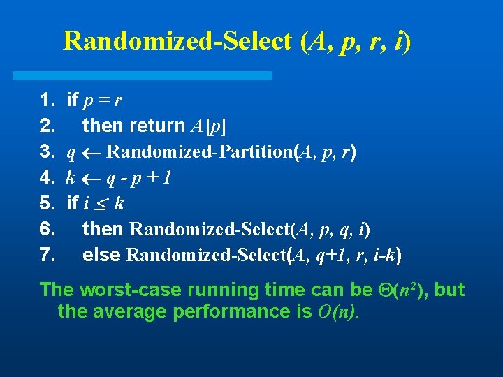
Randomized-Select (A, p, r, i) 1. 2. 3. 4. 5. 6. 7. if p = r then return A[p] q Randomized-Partition(A, p, r) k q-p+1 if i k then Randomized-Select(A, p, q, i) else Randomized-Select(A, q+1, r, i-k) The worst-case running time can be (n 2), but the average performance is O(n).

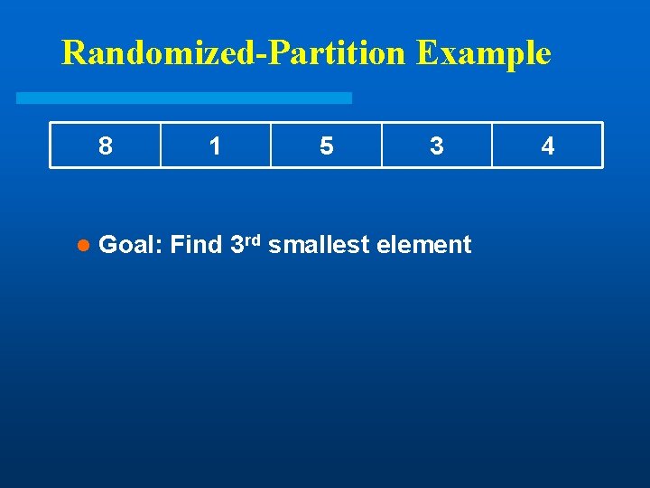
Randomized-Partition Example 8 l 1 5 3 Goal: Find 3 rd smallest element 4

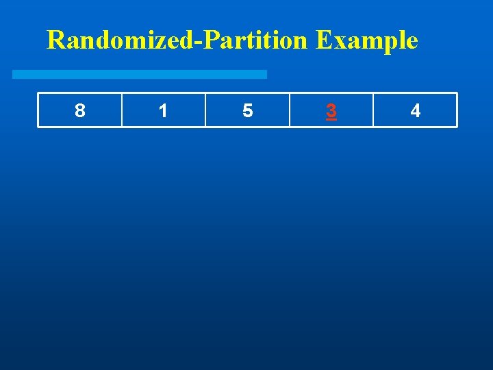
Randomized-Partition Example 8 1 5 3 4

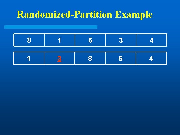
Randomized-Partition Example 8 1 5 3 4 1 3 8 5 4

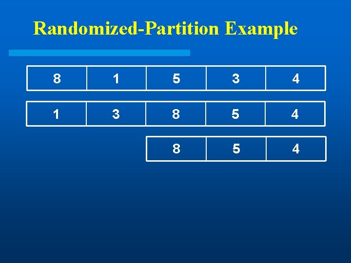
Randomized-Partition Example 8 1 5 3 4 1 3 8 5 4

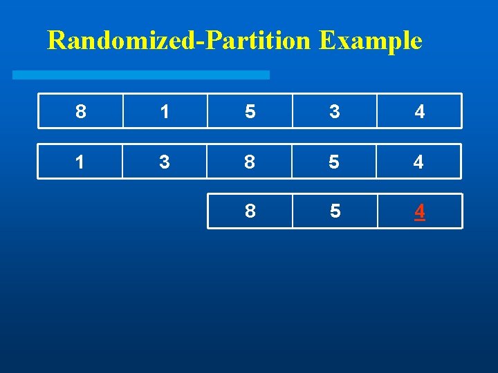
Randomized-Partition Example 8 1 5 3 4 1 3 8 5 4

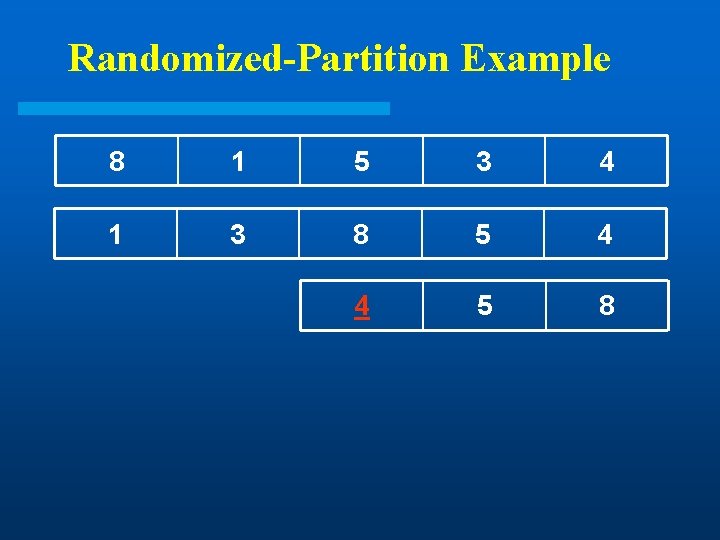
Randomized-Partition Example 8 1 5 3 4 1 3 8 5 4 4 5 8

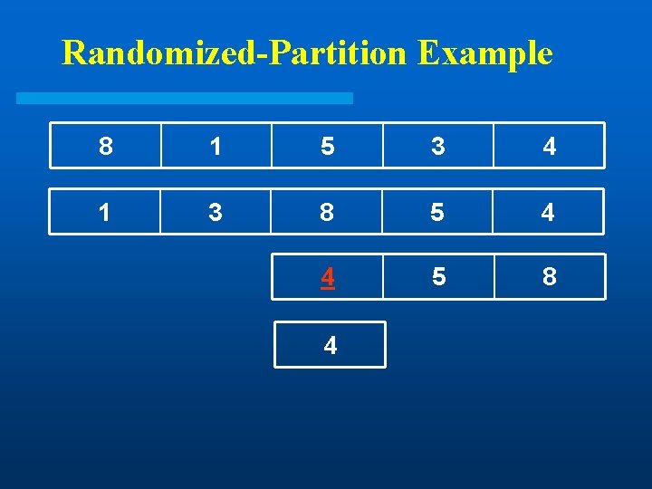
Randomized-Partition Example 8 1 5 3 4 1 3 8 5 4 4 5 8 4

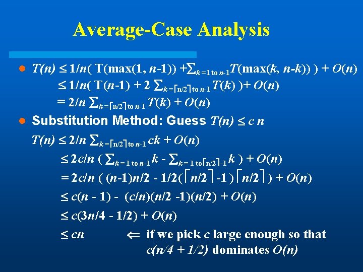
Average-Case Analysis T(n) 1/n( T(max(1, n-1)) + k =1 to n-1 T(max(k, n-k)) ) + O(n) 1/n( T(n-1) + 2 k = n/2 to n-1 T(k) )+ O(n) = 2/n k = n/2 to n-1 T(k) + O(n) l Substitution Method: Guess T(n) c n T(n) 2/n k = n/2 to n-1 ck + O(n) 2 c/n ( k = 1 to n-1 k - k = 1 to n/2 -1 k ) + O(n) = 2 c/n ( (n-1)n/2 - 1/2( n/2 -1 ) n/2 ) + O(n) c(n - 1) - (c/n)(n/2 -1)(n/2) + O(n) c(3 n/4 - 1/2) + O(n) cn if we pick c large enough so that c(n/4 + 1/2) dominates O(n) l

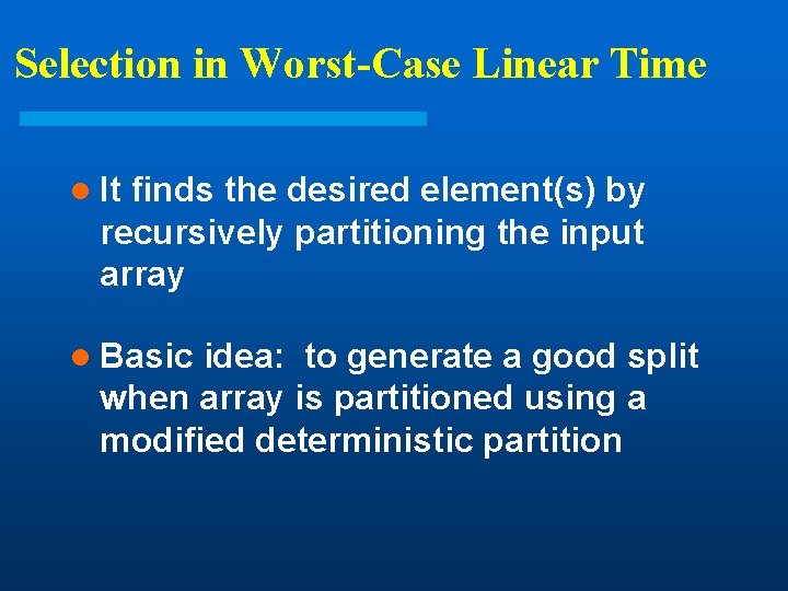
Selection in Worst-Case Linear Time l It finds the desired element(s) by recursively partitioning the input array l Basic idea: to generate a good split when array is partitioned using a modified deterministic partition

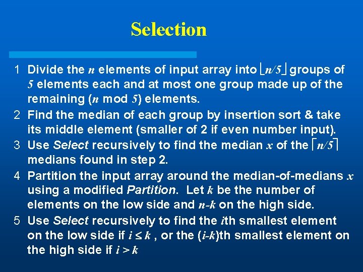
Selection 1 Divide the n elements of input array into n/5 groups of 5 elements each and at most one group made up of the remaining (n mod 5) elements. 2 Find the median of each group by insertion sort & take its middle element (smaller of 2 if even number input). 3 Use Select recursively to find the median x of the n/5 medians found in step 2. 4 Partition the input array around the median-of-medians x using a modified Partition. Let k be the number of elements on the low side and n-k on the high side. 5 Use Select recursively to find the ith smallest element on the low side if i k , or the (i-k)th smallest element on the high side if i > k

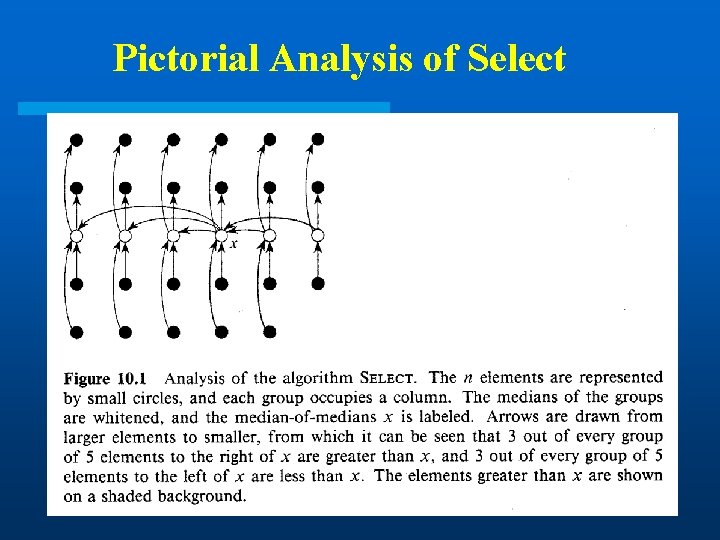
Pictorial Analysis of Select

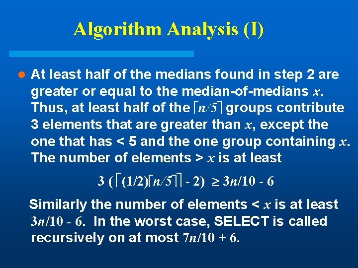
Algorithm Analysis (I) l At least half of the medians found in step 2 are greater or equal to the median-of-medians x. Thus, at least half of the n/5 groups contribute 3 elements that are greater than x, except the one that has < 5 and the one group containing x. The number of elements > x is at least 3 ( (1/2) n/5 - 2) 3 n/10 - 6 Similarly the number of elements < x is at least 3 n/10 - 6. In the worst case, SELECT is called recursively on at most 7 n/10 + 6.

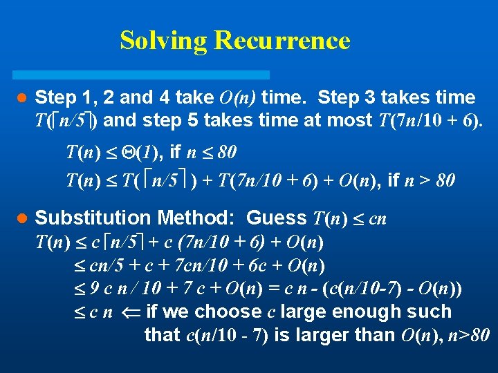
Solving Recurrence l Step 1, 2 and 4 take O(n) time. Step 3 takes time T( n/5 ) and step 5 takes time at most T(7 n/10 + 6). T(n) (1), if n 80 T(n) T( n/5 ) + T(7 n/10 + 6) + O(n), if n > 80 l Substitution Method: Guess T(n) cn T(n) c n/5 + c (7 n/10 + 6) + O(n) cn/5 + c + 7 cn/10 + 6 c + O(n) 9 c n / 10 + 7 c + O(n) = c n - (c(n/10 -7) - O(n)) c n if we choose c large enough such that c(n/10 - 7) is larger than O(n), n>80

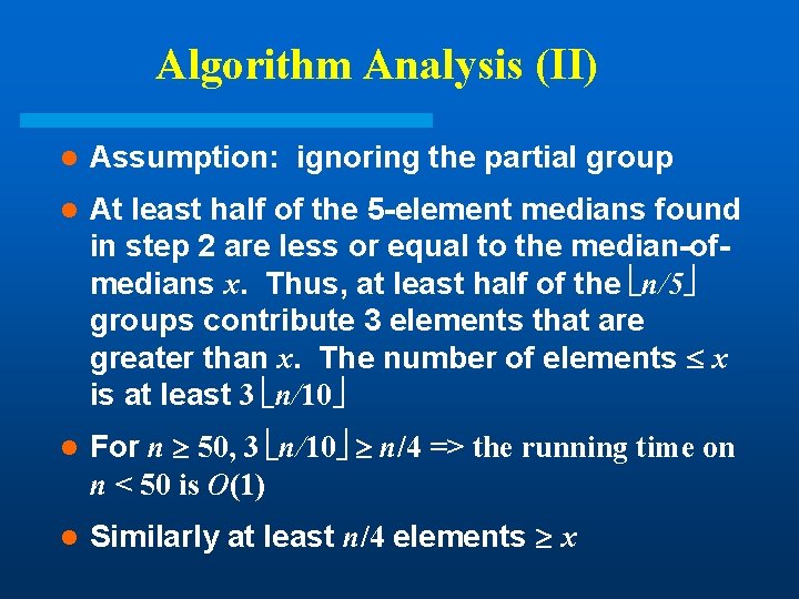
Algorithm Analysis (II) l Assumption: ignoring the partial group l At least half of the 5 -element medians found in step 2 are less or equal to the median-ofmedians x. Thus, at least half of the n/5 groups contribute 3 elements that are greater than x. The number of elements x is at least 3 n/10 l For n 50, 3 n/10 n/4 => the running time on n < 50 is O(1) l Similarly at least n/4 elements x

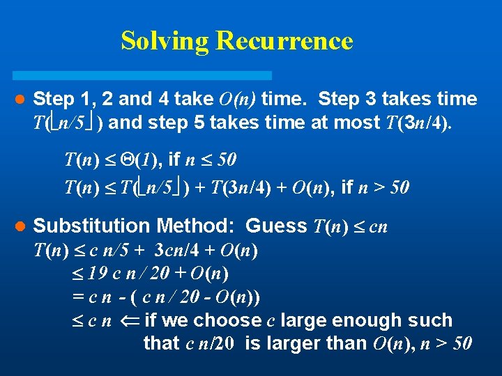
Solving Recurrence l Step 1, 2 and 4 take O(n) time. Step 3 takes time T( n/5 ) and step 5 takes time at most T(3 n/4). T(n) (1), if n 50 T(n) T( n/5 ) + T(3 n/4) + O(n), if n > 50 l Substitution Method: Guess T(n) cn T(n) c n/5 + 3 cn/4 + O(n) 19 c n / 20 + O(n) = c n - ( c n / 20 - O(n)) c n if we choose c large enough such that c n/20 is larger than O(n), n > 50

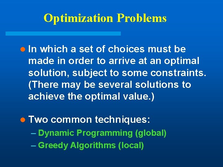
Optimization Problems l In which a set of choices must be made in order to arrive at an optimal solution, subject to some constraints. (There may be several solutions to achieve the optimal value. ) l Two common techniques: – Dynamic Programming (global) – Greedy Algorithms (local)

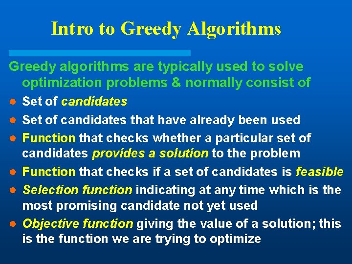
Intro to Greedy Algorithms Greedy algorithms are typically used to solve optimization problems & normally consist of l l l Set of candidates that have already been used Function that checks whether a particular set of candidates provides a solution to the problem Function that checks if a set of candidates is feasible Selection function indicating at any time which is the most promising candidate not yet used Objective function giving the value of a solution; this is the function we are trying to optimize

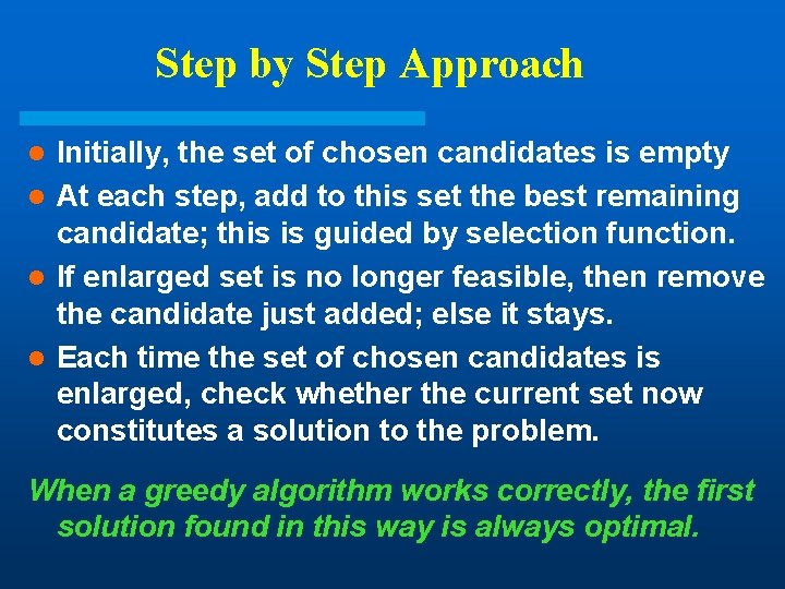
Step by Step Approach Initially, the set of chosen candidates is empty l At each step, add to this set the best remaining candidate; this is guided by selection function. l If enlarged set is no longer feasible, then remove the candidate just added; else it stays. l Each time the set of chosen candidates is enlarged, check whether the current set now constitutes a solution to the problem. l When a greedy algorithm works correctly, the first solution found in this way is always optimal.

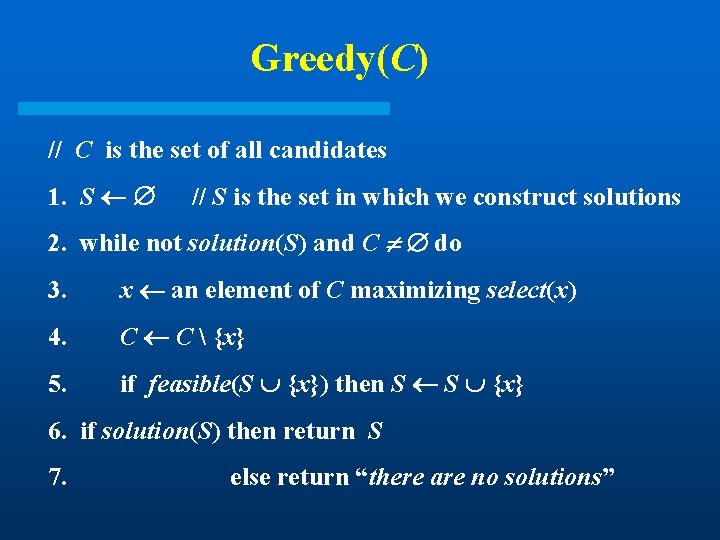
Greedy(C) // C is the set of all candidates 1. S // S is the set in which we construct solutions 2. while not solution(S) and C do 3. x an element of C maximizing select(x) 4. C C {x} 5. if feasible(S {x}) then S S {x} 6. if solution(S) then return S 7. else return “there are no solutions”

Analysis l The selection function is usually based on the objective function; they may be identical. But, often there are several plausible ones. l At every step, the procedure chooses the best morsel it can swallow, without worrying about the future. It never changes its mind: once a candidate is included in the solution, it is there for good; once a candidate is excluded, it’s never considered again. l Greedy algorithms do NOT always yield optimal solutions, but for many problems they do.

Examples of Greedy Algorithms l Scheduling – Activity Selection (Chap 17. 1) – Minimizing time in system – Deadline scheduling l Graph Algorithms – Minimum Spanning Trees (Chap 24) – Dijkstra’s (shortest path) Algorithm (Chap 25) l Other Heuristics – Coloring a graph – Traveling Salesman (Chap 37. 2) – Set-covering (Chap 37. 3)

Elements of Greedy Strategy Greedy-choice property: A global optimal solution can be arrived at by making locally optimal (greedy) choices l Optimal substructure: an optimal solution to the problem contains within it optimal solutions to sub-problems l – Be able to demonstrate that if A is an optimal solution containing s 1, then the set A’ = A - {s 1} is an optimal solution to a smaller problem w/o s 1. (See proof of Theorem 16. 1)

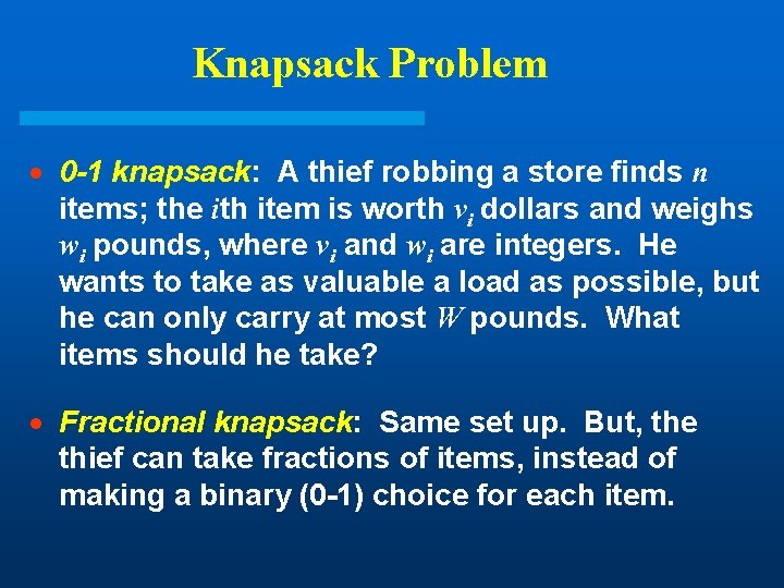
Knapsack Problem · 0 -1 knapsack: A thief robbing a store finds n items; the ith item is worth vi dollars and weighs wi pounds, where vi and wi are integers. He wants to take as valuable a load as possible, but he can only carry at most W pounds. What items should he take? · Fractional knapsack: Same set up. But, the thief can take fractions of items, instead of making a binary (0 -1) choice for each item.

Comparisons l Which problem exhibits greedy choice property? l Which one exhibits optimal-substructure property?

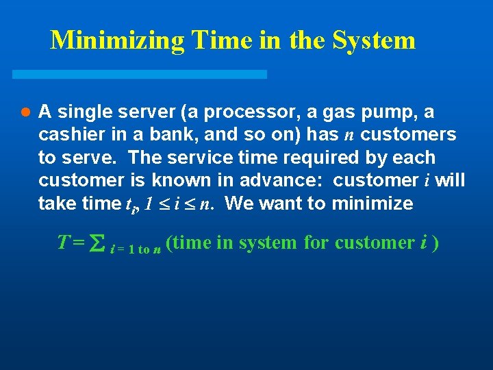
Minimizing Time in the System l A single server (a processor, a gas pump, a cashier in a bank, and so on) has n customers to serve. The service time required by each customer is known in advance: customer i will take time ti, 1 i n. We want to minimize T = i = 1 to n (time in system for customer i )

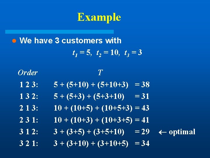
Example l We have 3 customers with t 1 = 5, t 2 = 10, t 3 = 3 Order 1 2 3: 1 3 2: 2 1 3: 2 3 1: 3 1 2: 3 2 1: T 5 + (5+10) + (5+10+3) = 38 5 + (5+3) + (5+3+10) = 31 10 + (10+5) + (10+5+3) = 43 10 + (10+3) + (10+3+5) = 41 3 + (3+5) + (3+5+10) = 29 3 + (3+10) + (3+10+5) = 34 optimal

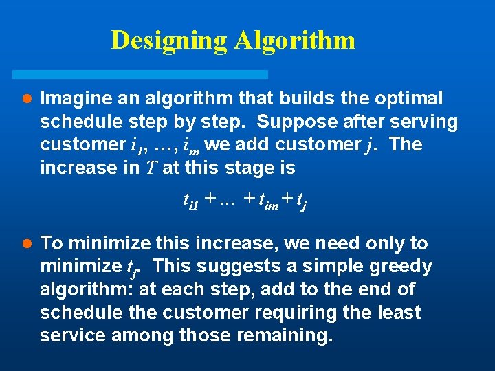
Designing Algorithm l Imagine an algorithm that builds the optimal schedule step by step. Suppose after serving customer i 1, …, im we add customer j. The increase in T at this stage is ti 1 + … + tim + tj l To minimize this increase, we need only to minimize tj. This suggests a simple greedy algorithm: at each step, add to the end of schedule the customer requiring the least service among those remaining.

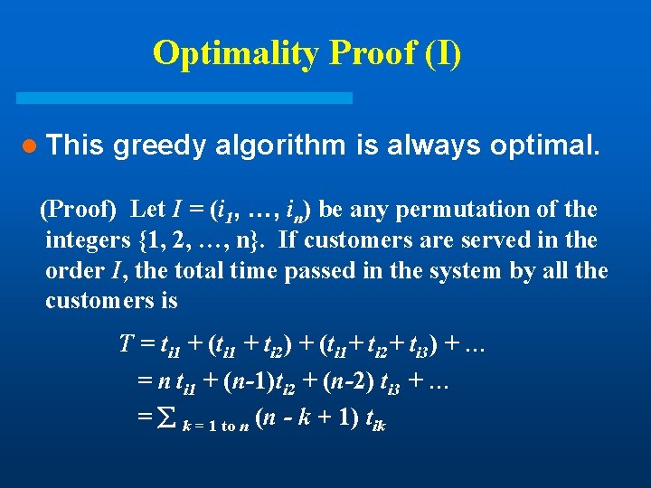
Optimality Proof (I) l This greedy algorithm is always optimal. (Proof) Let I = (i 1, …, in) be any permutation of the integers {1, 2, …, n}. If customers are served in the order I, the total time passed in the system by all the customers is T = ti 1 + (ti 1 + ti 2) + (ti 1+ ti 2+ ti 3) + … = n ti 1 + (n-1)ti 2 + (n-2) ti 3 + … = k = 1 to n (n - k + 1) tik

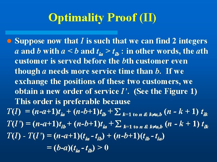
Optimality Proof (II) Suppose now that I is such that we can find 2 integers a and b with a < b and tia > tib : in other words, the ath customer is served before the bth customer even though a needs more service time than b. If we exchange the positions of these two customers, we obtain a new order of service I’. (See the Figure 1) This order is preferable because T(I) = (n-a+1)tia + (n-b+1)tib + k=1 to n & k a, b (n - k + 1) tik T(I’) = (n-a+1)tib + (n-b+1)tia + k=1 to n & k a, b (n - k + 1) tik T(I) - T(I’) = (n-a+1)(tia - tib) + (n-b+1)(tib - tia) = (b-a)(tia - tib) > 0 l

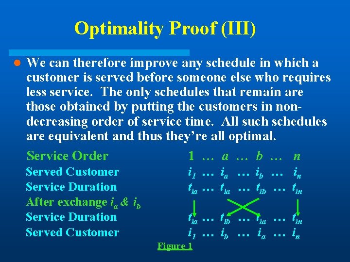
Optimality Proof (III) l We can therefore improve any schedule in which a customer is served before someone else who requires less service. The only schedules that remain are those obtained by putting the customers in nondecreasing order of service time. All such schedules are equivalent and thus they’re all optimal. Service Order 1 … a … b … n Served Customer Service Duration After exchange ia & ib Service Duration Served Customer i 1 … ia … ib … in tia … tib … tin tia … tib … tia … tin i 1 … ib … ia … in Figure 1

Optimization Problems l In which a set of choices must be made in order to arrive at an optimal (min/max) solution, subject to some constraints. (There may be several solutions to achieve an optimal value. ) l Two common techniques: – Dynamic Programming (global) – Greedy Algorithms (local)

Dynamic Programming l Similar to divide-and-conquer, it breaks problems down into smaller problems that are solved recursively. l In contrast, DP is applicable when the subproblems are not independent, i. e. when sub -problems share sub-problems. It solves every sub-problem just once and save the results in a table to avoid duplicated computation.

Elements of DP Algorithms Sub-structure: decompose problem into smaller sub-problems. Express the solution of the original problem in terms of solutions for smaller problems. l Table-structure: Store the answers to the subproblem in a table, because sub-problem solutions may be used many times. l Bottom-up computation: combine solutions on smaller sub-problems to solve larger subproblems, and eventually arrive at a solution to the complete problem. l

Applicability to Optimization Problems l Optimal sub-structure (principle of optimality): for the global problem to be solved optimally, each subproblem should be solved optimally. This is often violated due to sub-problem overlaps. Often by being “less optimal” on one problem, we may make a big savings on another sub-problem. l Small number of sub-problems: Many NP-hard problems can be formulated as DP problems, but these formulations are not efficient, because the number of subproblems is exponentially large. Ideally, the number of sub -problems should be at most a polynomial number.

Optimized Chain Operations l Determine the optimal sequence for performing a series of operations. (the general class of the problem is important in compiler design for code optimization & in databases for query optimization) l For example: given a series of matrices: A 1…An , we can “parenthesize” this expression however we like, since matrix multiplication is associative (but not commutative). l Multiply a p x q matrix A times a q x r matrix B, the result will be a p x r matrix C. (# of columns of A must be equal to # of rows of B. )

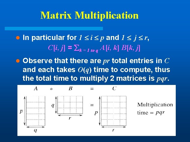
Matrix Multiplication l In particular for 1 i p and 1 j r, C[i, j] = k = 1 to q A[i, k] B[k, j] l Observe that there are pr total entries in C and each takes O(q) time to compute, thus the total time to multiply 2 matrices is pqr.

Chain Matrix Multiplication l Given a sequence of matrices A 1 A 2…An , and dimensions p 0 p 1…pn where Ai is of dimension pi-1 x pi , determine multiplication sequence that minimizes the number of operations. l This algorithm does not perform the multiplication, it just figures out the best order in which to perform the multiplication.

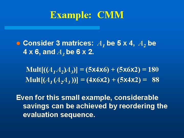
Example: CMM l Consider 3 matrices: A 1 be 5 x 4, A 2 be 4 x 6, and A 3 be 6 x 2. Mult[((A 1 A 2)A 3)] = (5 x 4 x 6) + (5 x 6 x 2) = 180 Mult[(A 1 (A 2 A 3 ))] = (4 x 6 x 2) + (5 x 4 x 2) = 88 Even for this small example, considerable savings can be achieved by reordering the evaluation sequence.

Naive Algorithm l If we have just 1 item, then there is only one way to parenthesize. If we have n items, then there are n-1 places where you could break the list with the outermost pair of parentheses, namely just after the first item, just after the 2 nd item, etc. and just after the (n-1)th item. l When we split just after the kth item, we create two sub-lists to be parenthesized, one with k items and the other with n-k items. Then we consider all ways of parenthesizing these. If there are L ways to parenthesize the left sub-list, R ways to parenthesize the right sub-list, then the total possibilities is L R.

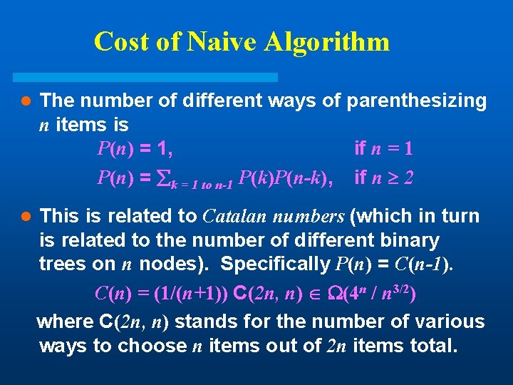
Cost of Naive Algorithm l The number of different ways of parenthesizing n items is P(n) = 1, if n = 1 P(n) = k = 1 to n-1 P(k)P(n-k), if n 2 l This is related to Catalan numbers (which in turn is related to the number of different binary trees on n nodes). Specifically P(n) = C(n-1). C(n) = (1/(n+1)) C(2 n, n) (4 n / n 3/2) where C(2 n, n) stands for the number of various ways to choose n items out of 2 n items total.

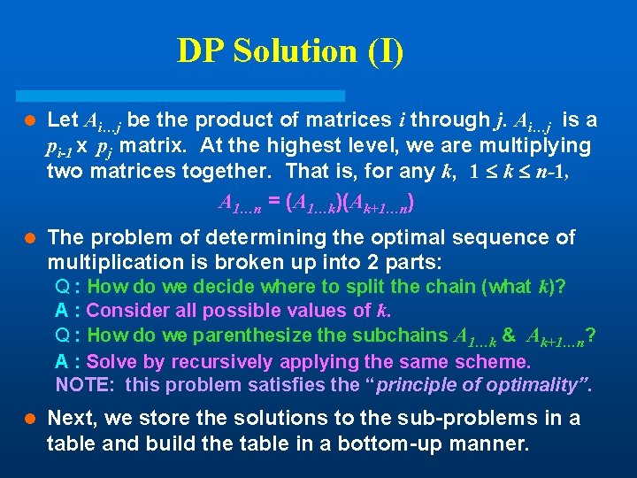
DP Solution (I) l Let Ai…j be the product of matrices i through j. Ai…j is a pi-1 x pj matrix. At the highest level, we are multiplying two matrices together. That is, for any k, 1 k n-1, A 1…n = (A 1…k)(Ak+1…n) l The problem of determining the optimal sequence of multiplication is broken up into 2 parts: Q : How do we decide where to split the chain (what k)? A : Consider all possible values of k. Q : How do we parenthesize the subchains A 1…k & Ak+1…n? A : Solve by recursively applying the same scheme. NOTE: this problem satisfies the “principle of optimality”. l Next, we store the solutions to the sub-problems in a table and build the table in a bottom-up manner.

DP Solution (II) For 1 i j n, let m[i, j] denote the minimum number of multiplications needed to compute Ai…j. l Example: Minimum number of multiplies for A 3… 7 l l In terms of pi , the product A 3… 7 has dimensions ____.

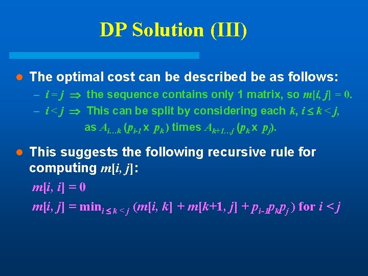
DP Solution (III) l The optimal cost can be described be as follows: – i = j the sequence contains only 1 matrix, so m[i, j] = 0. – i < j This can be split by considering each k, i k < j, as Ai…k (pi-1 x pk ) times Ak+1…j (pk x pj). l This suggests the following recursive rule for computing m[i, j]: m[i, i] = 0 m[i, j] = mini k < j (m[i, k] + m[k+1, j] + pi-1 pkpj ) for i < j

Computing m[i, j] l For a specific k, (Ai …Ak)( Ak+1 … Aj) = m[i, j] = mini k < j (m[i, k] + m[k+1, j] + pi-1 pkpj )

Computing m[i, j] l For a specific k, (Ai …Ak)( Ak+1 … Aj) = Ai…k( Ak+1 … Aj) (m[i, k] mults) m[i, j] = mini k < j (m[i, k] + m[k+1, j] + pi-1 pkpj )

Computing m[i, j] l For a specific k, (Ai …Ak)( Ak+1 … Aj) = Ai…k( Ak+1 … Aj) (m[i, k] mults) = Ai…k Ak+1…j (m[k+1, j] mults) m[i, j] = mini k < j (m[i, k] + m[k+1, j] + pi-1 pkpj )

Computing m[i, j] l For a specific k, (Ai …Ak)( Ak+1 … Aj) = Ai…k( Ak+1 … Aj) (m[i, k] mults) = Ai…k Ak+1…j (m[k+1, j] mults) = Ai…j (pi-1 pk pj mults) m[i, j] = mini k < j (m[i, k] + m[k+1, j] + pi-1 pkpj )

Computing m[i, j] l For a specific k, (Ai …Ak)( Ak+1 … Aj) = Ai…k( Ak+1 … Aj) (m[i, k] mults) = Ai…k Ak+1…j (m[k+1, j] mults) = Ai…j (pi-1 pk pj mults) l For solution, evaluate for all k and take minimum. m[i, j] = mini k < j (m[i, k] + m[k+1, j] + pi-1 pkpj )

Matrix-Chain-Order(p) 1. n length[p] - 1 2. for i 1 to n // initialization: O(n) time 3. do m[i, i] 0 4. for L 2 to n // L = length of sub-chain 5. do for i 1 to n - L+1 6. do j i + L - 1 7. m[i, j] 8. for k i to j - 1 9. do q m[i, k] + m[k+1, j] + pi-1 pk pj 10. if q < m[i, j] 11. then m[i, j] q 12. s[i, j] k 13. return m and s

Analysis l The array s[i, j] is used to extract the actual sequence (see next). l There are 3 nested loops and each can iterate at most n times, so the total running time is (n 3).

Extracting Optimum Sequence l Leave a split marker indicating where the best split is (i. e. the value of k leading to minimum values of m[i, j]). We maintain a parallel array s[i, j] in which we store the value of k providing the optimal split. l If s[i, j] = k, the best way to multiply the subchain Ai…j is to first multiply the sub-chain Ai…k and then the sub-chain Ak+1…j , and finally multiply them together. Intuitively s[i, j] tells us what multiplication to perform last. We only need to store s[i, j] if we have at least 2 matrices & j > i.

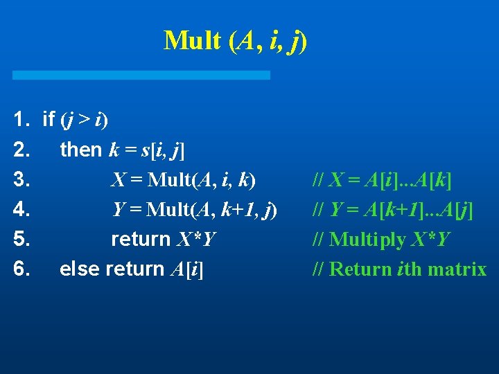
Mult (A, i, j) 1. if (j > i) 2. then k = s[i, j] 3. X = Mult(A, i, k) 4. Y = Mult(A, k+1, j) 5. return X*Y 6. else return A[i] // X = A[i]. . . A[k] // Y = A[k+1]. . . A[j] // Multiply X*Y // Return ith matrix

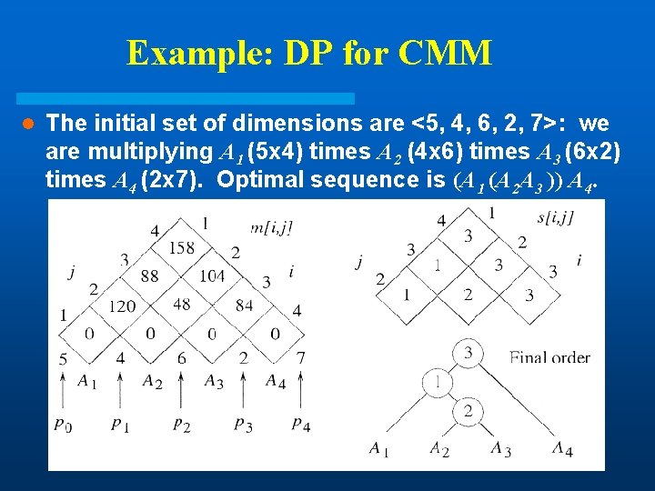
Example: DP for CMM l The initial set of dimensions are <5, 4, 6, 2, 7>: we are multiplying A 1 (5 x 4) times A 2 (4 x 6) times A 3 (6 x 2) times A 4 (2 x 7). Optimal sequence is (A 1 (A 2 A 3 )) A 4.

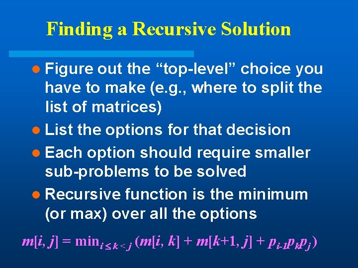
Finding a Recursive Solution l Figure out the “top-level” choice you have to make (e. g. , where to split the list of matrices) l List the options for that decision l Each option should require smaller sub-problems to be solved l Recursive function is the minimum (or max) over all the options m[i, j] = mini k < j (m[i, k] + m[k+1, j] + pi-1 pkpj )

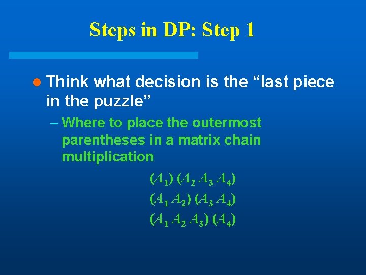
Steps in DP: Step 1 l Think what decision is the “last piece in the puzzle” – Where to place the outermost parentheses in a matrix chain multiplication (A 1) (A 2 A 3 A 4) (A 1 A 2) (A 3 A 4) (A 1 A 2 A 3) (A 4)

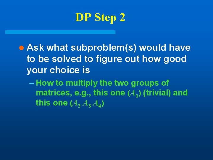
DP Step 2 l Ask what subproblem(s) would have to be solved to figure out how good your choice is – How to multiply the two groups of matrices, e. g. , this one (A 1) (trivial) and this one (A 2 A 3 A 4)

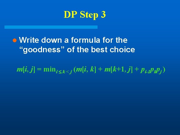
DP Step 3 l Write down a formula for the “goodness” of the best choice m[i, j] = mini k < j (m[i, k] + m[k+1, j] + pi-1 pkpj )

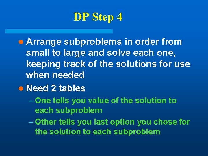
DP Step 4 l Arrange subproblems in order from small to large and solve each one, keeping track of the solutions for use when needed l Need 2 tables – One tells you value of the solution to each subproblem – Other tells you last option you chose for the solution to each subproblem

Matrix-Chain-Order(p) 1. n length[p] - 1 2. for i 1 to n // initialization: O(n) time 3. do m[i, i] 0 4. for L 2 to n // L = length of sub-chain 5. do for i 1 to n - L+1 6. do j i + L - 1 7. m[i, j] 8. for k i to j - 1 9. do q m[i, k] + m[k+1, j] + pi-1 pk pj 10. if q < m[i, j] 11. then m[i, j] q 12. s[i, j] k 13. return m and s

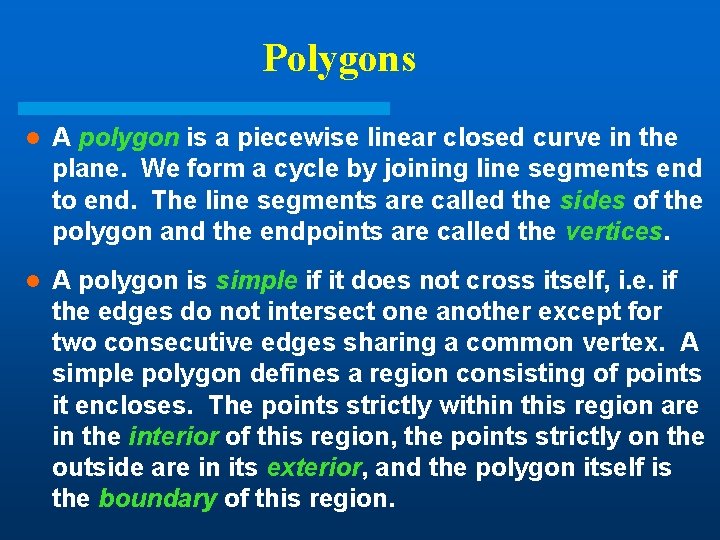
Polygons l A polygon is a piecewise linear closed curve in the plane. We form a cycle by joining line segments end to end. The line segments are called the sides of the polygon and the endpoints are called the vertices. l A polygon is simple if it does not cross itself, i. e. if the edges do not intersect one another except for two consecutive edges sharing a common vertex. A simple polygon defines a region consisting of points it encloses. The points strictly within this region are in the interior of this region, the points strictly on the outside are in its exterior, and the polygon itself is the boundary of this region.

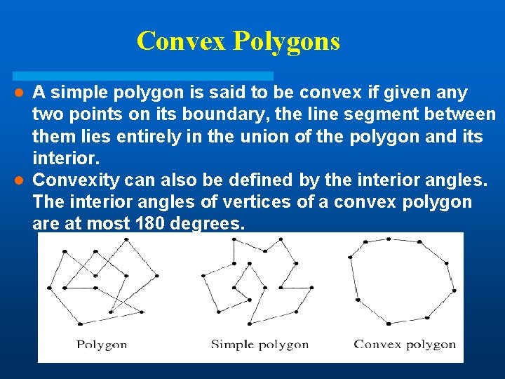
Convex Polygons A simple polygon is said to be convex if given any two points on its boundary, the line segment between them lies entirely in the union of the polygon and its interior. l Convexity can also be defined by the interior angles. The interior angles of vertices of a convex polygon are at most 180 degrees. l

Triangulations Given a convex polygon, assume that its vertices are labeled in counterclockwise order P=<v 0, …, vn-1>. Assume that indexing of vertices is done modulo n, so v 0 = vn. This polygon has n sides, (vi-1 , vi ). l Given two nonadjacent vj , where i < j, the line segment (vi , vj ) is a chord. (If the polygon is simple but not convex, a segment must also lie entirely in the interior of P for it to be a chord. ) Any chord subdivides the polygon into two polygons. l A triangulation of a convex polygon is a maximal set T of chords. Every chord that is not in T intersects the interior of some chord in T. Such a set of chords subdivides interior of a polygon into set of triangles. l

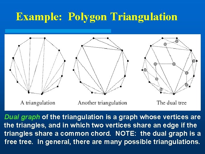
Example: Polygon Triangulation Dual graph of the triangulation is a graph whose vertices are the triangles, and in which two vertices share an edge if the triangles share a common chord. NOTE: the dual graph is a free tree. In general, there are many possible triangulations.

Minimum-Weight Convex Polygon Triangulation l The number of possible triangulations is exponential in n, the number of sides. The “best” triangulation depends on the applications. l Our problem: Given a convex polygon, determine the triangulation that minimizes the sum of the perimeters of its triangles. l Given three distinct vertices, vi , vj and vk , we define the weight of the associated triangle by the weight function w(vi , vj , vk) = |vi vj | + |vj vk | + |vk vi |, where |vi vj | denotes length of the line segment (vi , vj ).

Correspondence to Binary Trees In MCM, the associated binary tree is the evaluation tree for the multiplication, where the leaves of the tree correspond to the matrices, and each node of the tree is associated with a product of a sequence of two or more matrices. l Consider an (n+1)-sided convex polygon, P=<v 0, …, vn> and fix one side of the polygon, (v 0 , vn). Consider a rooted binary tree whose root node is the triangle containing side (v 0 , vn), whose internal nodes are the nodes of the dual tree, and whose leaves correspond to the remaining sides of the tree. The partitioning of a polygon into triangles is equivalent to a binary tree with n-1 leaves, and vice versa. l

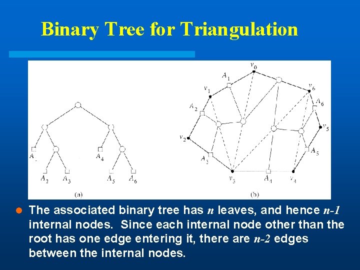
Binary Tree for Triangulation l The associated binary tree has n leaves, and hence n-1 internal nodes. Since each internal node other than the root has one edge entering it, there are n-2 edges between the internal nodes.

Lemma l. A triangulation of a simple polygon has n-2 triangles and n-3 chords. (Proof) The result follows directly from the previous figure. Each internal node corresponds to one triangle and each edge between internal nodes corresponds to one chord of triangulation. If we consider an n-vertex polygon, then we’ll have n-1 leaves, and thus n-2 internal nodes (triangles) and n-3 edges (chords).

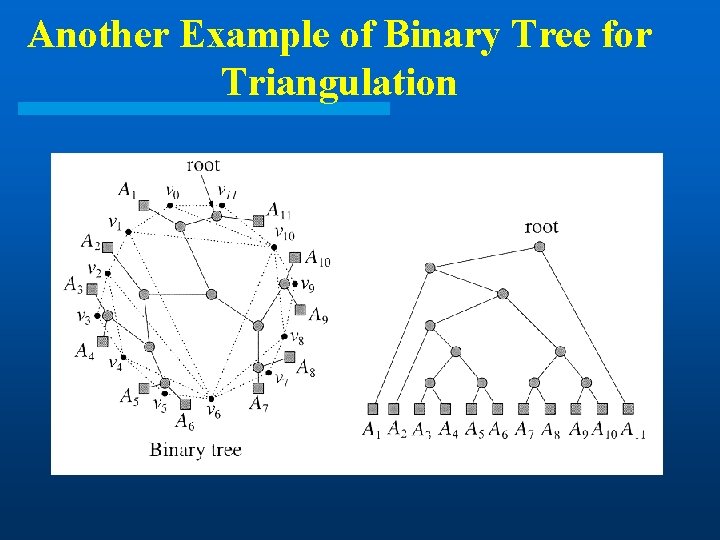
Another Example of Binary Tree for Triangulation

DP Solution (I) l For 1 i j n, let t[i, j] denote the minimum weight triangulation for the subpolygon <vi-1, vi , …, vj>. l We start with vi-1 rather than vi, to keep the structure as similar as possible to the matrix chain multiplication problem. v 5 v 4 v 3 Min. weight triangulation = t[2, 5] v 6 v 2 v 0 v 1

DP Solution (II) l Observe: if we can compute t[i, j] for all i and j (1 i j n), then the weight of minimum weight triangulation of the entire polygon will be t[1, n]. l For the basis case, the weight of the trivial 2 -sided polygon is zero, implying that t[i, i] = 0 (line (vi-1, vi)).

DP Solution (III) l In general, to compute t[i, j], consider the subpolygon <vi-1, vi , …, vj>, where i j. One of the chords of this polygon is the side (vi-1, vj). We may split this subpolygon by introducting a triangle whose base is this chord, and whose third vertex is any vertex vk, where i k j-1. This subdivides the polygon into 2 subpolygons <vi-1, . . . vk> & <vk+1, . . . vj>, whose minimum weights are t[i, k] and t[k+1, j]. l We have following recursive rule for computing t[i, j]: t[i, i] = 0 t[i, j] = mini k j-1 (t[i, k] + t[k+1, j] + w(vi-1 vkvj )) for i < k

Weighted-Polygon-Triangulation(V) 1. n length[V] - 1 // V = <v 0 , v 1 , …, vn> 2. for i 1 to n // initialization: O(n) time 3. do t[i, i] 0 4. for L 2 to n // L = length of sub-chain 5. do for i 1 to n-L+1 6. do j i + L - 1 7. t[i, j] 8. for k i to j - 1 9. do q t[i, k] + t[k+1, j] + w(vi-1 , vk , vj) 10. if q < t[i, j] 11. then t[i, j] q 12. s[i, j] k 13. return t and s

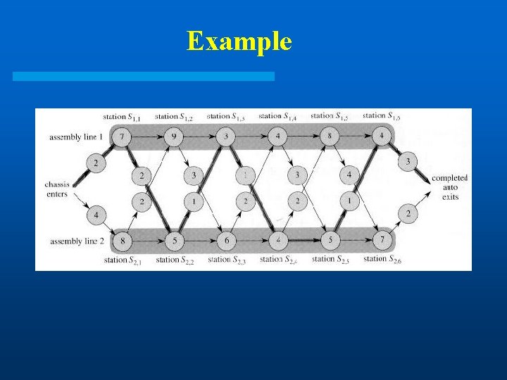
Assembly-Line Scheduling l Two parallel assembly lines in a factory, lines 1 and 2 l Each line has n stations Si, 1…Si, n l For each j, S 1, j does the same thing as S 2, j , but it may take a different amount of assembly time ai, j l Transferring away from line i after stage j costs ti, j l Also entry time ei and exit time xi at beginning and end

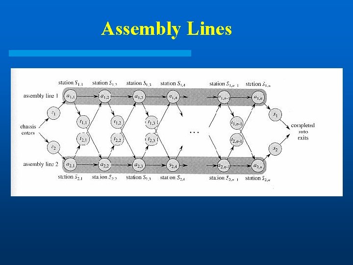
Assembly Lines

Finding Subproblem l Pick some convenient stage of the process – Say, just before the last station l What’s the next decision to make? – Whether the last station should be S 1, n or S 2, n l What do you need to know to decide which option is better? – What the fastest times are for S 1, n & S 2, n

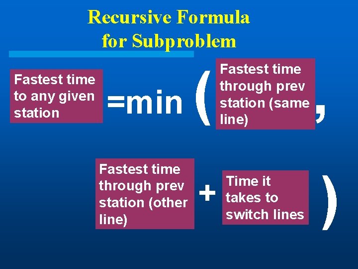
Recursive Formula for Subproblem Fastest time to any given station =min Fastest time through prev station (other line) ( + Fastest time through prev station (same line) Time it takes to switch lines , )

Recursive Formula (II) l Let fi [ j] denote the fastest possible time to get the chassis through S i, j l Have the following formulas: f 1[ 1] = e 1 + a 1, 1 f 1[ j] = min( f 1[ j-1] + a 1, j, f 2 [ j-1]+t 2, j-1+ a 1, j ) l Total time: f * = min( f 1[n] + x 1, f 2 [ n]+x 2)

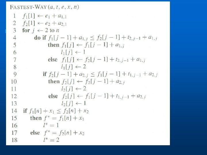
Analysis l Only loop is lines 3 -13 which iterate n -1 times: Algorithm is O(n). l The array l records which line is used for each station number

Example