Introduction to Scientific Computing A Matrix Vector Approach

Introduction to Scientific Computing -- A Matrix Vector Approach Using Matlab Written by Charles F. Van Loan 陈文斌 Wbchen@fudan. edu. cn 复旦大学

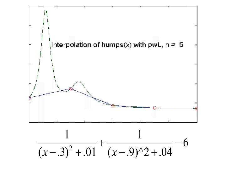
Chapter 3 Piecewise Polynomial Interpolation • Piecewise Linear Interpolation • Piecewise Cubic Hermite Interpolation • Cubic Splines

Piecewise Linear Interpolation 1 0. 8 0. 6 0. 4 0. 2 0 -0. 2 -0. 4 -0. 6 -0. 8 -1 0 1 2 3 4 5 6 7

Piecewise Linear

for i=1: n-1 b(i)=(y(i+1)- y(i))/ (x(i+1)- x(i)); end b=(y(2: n)-y(1: n-1)). /(x(2: n)-x(1: n 1)) b=diff(y). /diff(x) Test code z=linspace(0, 1, 9); [a, b]=pw. L(z, sin(2*pi*z)); function [a, b] = pw. L(x, y) n = length(x); a = y(1: n-1); b = diff(y). / diff(x);

Evalution Problem: if z==x(n) i =n-1; else i=sum(x<=z); end

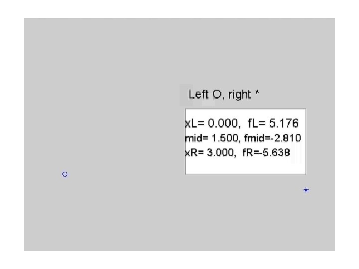
Binary search mid = floor((Left+Right)/2); If z<x(mid) Right=mid; Else Left =mid; end

function i = Locate(x, z, g) % g (1<=g<=n-1) is an optional input parameter % search for i begins, the value i=g is tried. if nargin==3 if (x(g)<=z) & (z<=x(g+1)) i = g; return end; end n = length(x); if z = = x(n) i = n-1; else Left = 1; Right = n; while Right > Left+1 Binary_search end g: guss

function LVals = pw. LEval(a, b, x, z. Vals) % Evaluates the piecewise linear polynomial defined by the column %(n-1)-vectors m = length(z. Vals); LVals = zeros(m, 1); g = 1; for j=1: m i = Locate(x, z. Vals(j), g); LVals(j) = a(i) + b(i)*(z. Vals(j)-x(i)); g = i; end m-vector

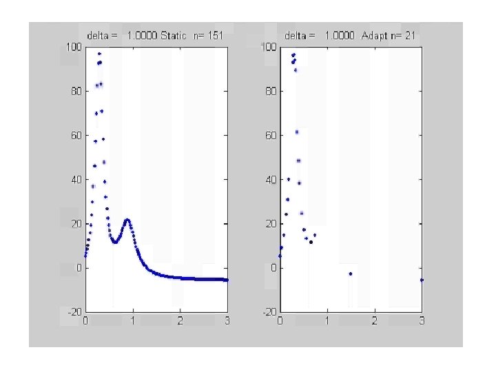
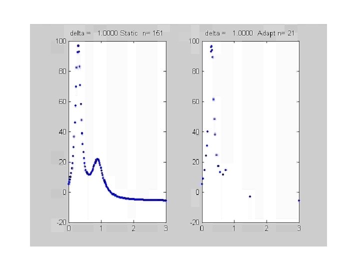
A priori determination of breakpoints Static

Adaptive Piecewise Linear Interpolation Problem

Adaptive Piecewise Linear Interpolation acceptable or

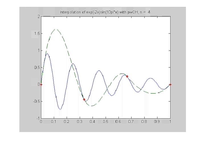
Piecewise Cubic Hermit Interpolation

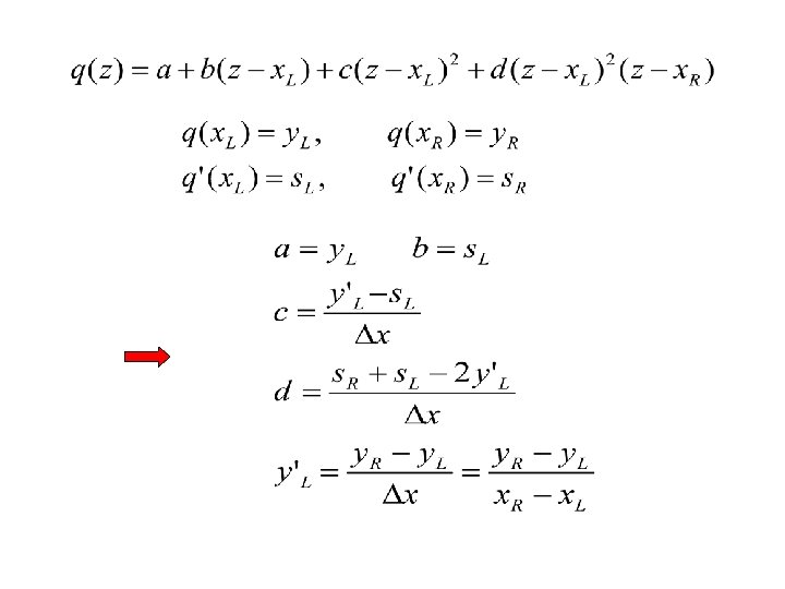
Hermit cubic interpolant

Piecewise cubic polynomial For i=1: n-1 [a(i), b(i), c(i), d(i)=Hcubic(x(i), y(i), s(i), x(i+1), y(i+1), s(i+1)) End

function [a, b, c, d] = pw. C(x, y, s) % Piecewise cubic Hermite interpolation. n = length(x); a = y(1: n-1); b = s(1: n-1); Dx = diff(x); Dy = diff(y); yp = Dy. / Dx; c = (yp - s(1: n-1)). / Dx; d = (s(2: n) + s(1: n-1) - 2*yp). / (Dx. * Dx); x, y, s: vector

Evaluation function Cvals = pw. CEval(a, b, c, d, x, z. Vals) m = length(z. Vals); Cvals = zeros(m, 1); g=1; for j=1: m i = Locate(x, z. Vals(j), g); Locate Cvals(j) = d(i)*(z. Vals(j)-x(i+1)) + c(i); Cvals(j) = Cvals(j)*(z. Vals(j)-x(i)) + b(i); Cvals(j) = Cvals(j)*(z. Vals(j)-x(i)) + a(i); g = i; end Cubic version of Horner. N

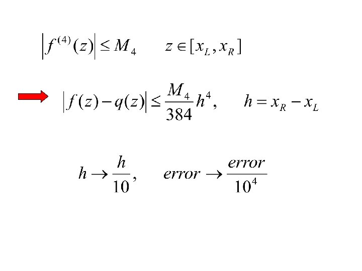
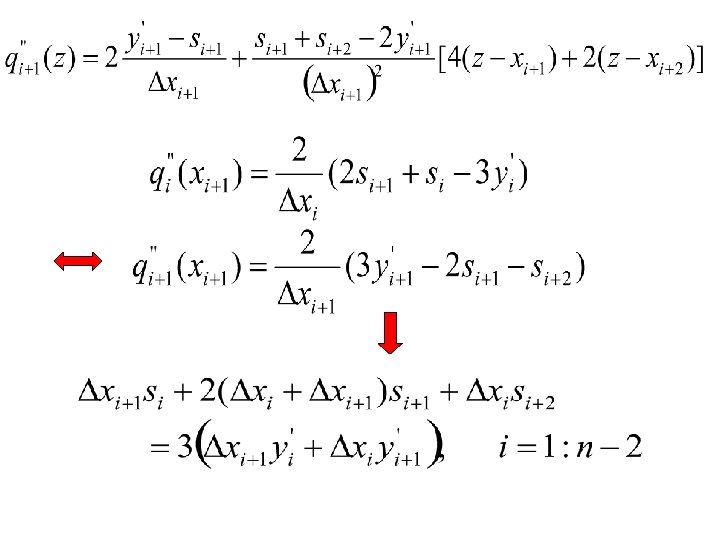
Cubic spline interpolant Given with find a piecewise cubic interpolant with the property that S, S' and S'' are continuous. Why need spline?

Continuity at the interior knots

tridiagonal

choice

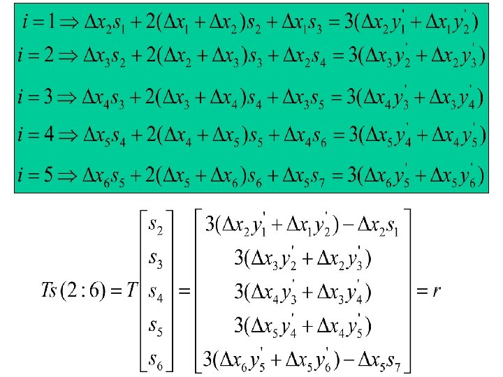
n=length(x); Dx=diff(x); yp=diff(y). /Dx; T=zeros(n-2, n-2); r=zeros(n-2, 1); for i=2: n-3 T(i, i)=2(Dx(i)+Dx(i+1)); T(i, i-1)=Dx(i+1); T(i, i+1)=Dx(i); r(i)=3(Dx(i+1)*yp(i)+Dx(i)*yp(i+1)); end Help diag

The complete spline

T(1, 1)=2*(Dx(1)+Dx(2)); T(1, 2)=Dx(1); r(1)=3*(Dx(2)*yp(1)+Dx(1)*yp(2))-Dx(2)*mu. L; T(n-2, n-2)=2*(Dx(n-2)+Dx(n-1)); T(n-2, n-3)=Dx(n-1); r(n-2)=3*(Dx(n-1)*yp(n-2)+Dx(n-2)*yp(n-1))-Dx(n-2)*mu. R; s=[mu. L; Tr(1: n-2); mu. R];

The Natural Spline

T(1, 1) = 2*Dx(1) + 1. 5*Dx(2); T(1, 2) = Dx(1); r(1) = 1. 5*Dx(2)*yp(1) + 3*Dx(1)*yp(2) + Dx(1)*Dx(2)*mu. L/4; T(n-2, n-2) = 1. 5*Dx(n-2)+2*Dx(n-1); T(n-2, n-3) = Dx(n-1); r(n-2) = 3*Dx(n-1)*yp(n-2) + 1. 5*Dx(n-2)*yp(n-1)- … Dx(n-1)*Dx(n-2)*mu. R/4; stilde = Tr; s 1 = (3*yp(1) - stilde(1) - mu. L*Dx(1)/2)/2; sn = (3*yp(n-1) - stilde(n-2) + mu. R*Dx(n-1)/2)/2; s = [s 1; stilde; sn];

The Not-a-Knot Spline

q = Dx(1)*Dx(1)/Dx(2); T(1, 1) = 2*Dx(1) +Dx(2) + q; T(1, 2) = Dx(1) + q; r(1) = Dx(2)*yp(1) + Dx(1)*yp(2)+2*yp(2)*(q+Dx(1)); q = Dx(n-1)*Dx(n-1)/Dx(n-2); T(n-2, n-2) = 2*Dx(n-1) + Dx(n-2)+q; T(n-2, n-3) = Dx(n-1)+q; r(n-2) = Dx(n-1)*yp(n-2) + Dx(n-2)*yp(n-1) … +2*yp(n-2)*(Dx(n-1)+q); stilde = Tr; s 1 = -stilde(1)+2*yp(1); s 1 = s 1 + ((Dx(1)/Dx(2))^2)*(stilde(1)+stilde(2)-2*yp(2)); sn = -stilde(n-2) +2*yp(n-1); sn = sn+((Dx(n-1)/Dx(n-2))^2)*(stilde(n-3) … +stilde(n-2)-2*yp(n-2)); s = [s 1; stilde; sn];

function [a, b, c, d] = Cubic. Spline(x, y, derivative, mu. L, mu. R) % Cubic spline interpolation with prescribed end conditions. % Usage: % [a, b, c, d] = Cubic. Spline(x, y, 1, mu. L, mu. R) % S'(x(1)) = mu. L, S'(x(n)) = mu. R % [a, b, c, d] = Cubic. Spline(x, y, 2, mu. L, mu. R) % S''(x(1)) = mu. L, S''(x(n)) = mu. R % [a, b, c, d] = Cubic. Spline(x, y) % S'''(z) continuous at x(2) and x(n-1)

10 10 10 -4 10 -6 10 -8 10 -10 10 -12 0 0. 5 Knot Spacing = 0. 050 1 10 -4 -6 -8 -10 -12 0 Not-a-knot spline error 0. 5 Knot Spacing = 0. 005 1

1. 5 1 0. 5 0 -0. 5 -1 0 1 2 3 4 5 6 7 Bad end conditions 8 9 10

Matlab Spline Tools n = 9 Spline Interpolant of atan(x) 1. 5 z=linspace(-5, 5); 1 x=linspace(-5, 5, 9); y=atan(x); Svals=spline(x, y, z); plot(z, Svals) 0. 5 0 -0. 5 -1 -1. 5 -5 -4 -3 -2 -1 0 1 2 Not-a-knot spline 3 4 5

pp-representation x=linspace(-5, 5, 9); y=atan(x); pp-representation S=spline(x, y); z=linspace(-5, 5); Svals=ppval(S, z) plot(z, Svals) [x, rho, L, k]=unmkpp(S) The coefficients of the local polynomials are assembled in an L-by-k matrix rho

drho = [3*rho(: , 1) 2*rho(: , 2) rho(: , 3)]; d. S = mkpp(x, drho); V = PPVAL(PP, XX) returns the value at the points XX of the piecewise polynomial contained in PP, as constructed by SPLINE or the spline utility z = linspace(-5, 5); Svals = ppval(S, z); d. Svals = ppval(d. S, z);

Derivative of n = 9 Spline Interpolant of atan(x) 1 0. 9 0. 8 0. 7 0. 6 0. 5 0. 4 0. 3 0. 2 0. 1 0 -5 -4 -3 -2 -1 0 1 2 3 4 5

n = 9; x = linspace(-5, 5, n); y = atan(x); S = spline(x, y); [x, rho, L, k] = unmkpp(S); drho = [3*rho(: , 1) 2*rho(: , 2) rho(: , 3)]; d. S = mkpp(x, drho); z = linspace(-5, 5); Svals = ppval(S, z); d. Svals = ppval(d. S, z); atanvals = atan(z); Figure; plot(z, atanvals, z, Svals, x, y, '*'); title(sprintf('n = %2. 0 f Spline Interpolant of atan(x)', n)) datanvals = ones(size(z)). /(1 + z. *z); figure plot(z, datanvals, z, d. Svals) title(sprintf('Derivative of n = %2. 0 f Spline Interpolant of atan(x)', n))