Introduction to SAS Essentials Mastering SAS for Data

Introduction to SAS Essentials Mastering SAS for Data Analytics Alan Elliott and Wayne Woodward 1 SAS ESSENTIALS -- Elliott & Woodward

Chapter 16: LOGISTIC REGRESSION 2 SAS ESSENTIALS -- Elliott & Woodward

LEARNING OBJECTIVES • To be able to perform a logistic analysis using PROC LOGISTIC • To be able to create a SAS® program that will perform a simple logistic analysis • To be able to create a SAS program that will perform multiple logistic analyses • To be able to use SAS to assess a model's fit and predictive ability 3 SAS ESSENTIALS -- Elliott & Woodward

Binary Logistic Regression � Binary logistic regression models are based on a dependent variable that can take on only one of two values, such as presence or absence of a disease, deceased or not deceased, married or unmarried, and so on. In this setting, the independent (sometimes called explanatory or predictor) variables are used for predicting the probability of occurrence of an outcome (such as mortality). 4 SAS ESSENTIALS -- Elliott & Woodward

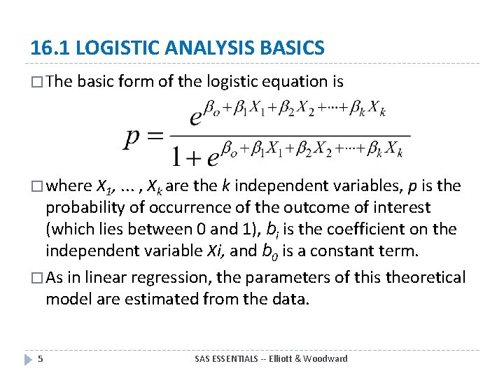
16. 1 LOGISTIC ANALYSIS BASICS � The basic form of the logistic equation is � where X 1, . . . , Xk are the k independent variables, p is the probability of occurrence of the outcome of interest (which lies between 0 and 1), bi is the coefficient on the independent variable Xi, and b 0 is a constant term. � As in linear regression, the parameters of this theoretical model are estimated from the data. 5 SAS ESSENTIALS -- Elliott & Woodward

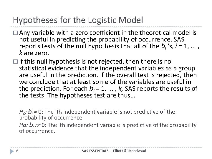
Hypotheses for the Logistic Model � Any variable with a zero coefficient in theoretical model is not useful in predicting the probability of occurrence. SAS reports tests of the null hypothesis that all of the bi 's, i = 1, . . . , k are zero. � lf this null hypothesis is not rejected, then there is no statistical evidence that the independent variables as a group are useful in the prediction. lf the overall test is rejected, then we conclude that at least some of the variables are useful in the prediction. For each bi = 1, . . . , k, SAS reports the results of the tests. The hypotheses test are thus… H 0: bi = 0: The ith independent variable is not predictive of the probability of occurrence. Ha: bi : 0: The ith independent variable is predictive of the probability of occurrence. 6 SAS ESSENTIALS -- Elliott & Woodward

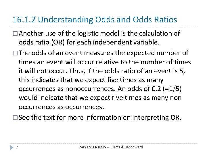
16. 1. 2 Understanding Odds and Odds Ratios � Another use of the logistic model is the calculation of odds ratio (OR) for each independent variable. � The odds of an event measures the expected number of times an event will occur relative to the number of times it will not occur. Thus, if the odds ratio of an event is 5, this indicates that we expect five times as many occurrences as nonoccurrences. An odds of 0. 2 (=1/5) would indicate that we expect five times as many non occurrences as occurrences. � See the text for more information on interpreting OR. 7 SAS ESSENTIALS -- Elliott & Woodward

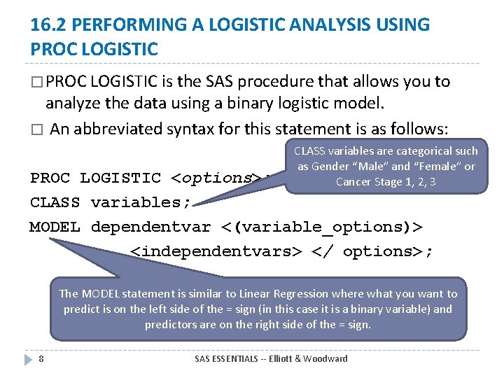
16. 2 PERFORMING A LOGISTIC ANALYSIS USING PROC LOGISTIC � PROC LOGISTIC is the SAS procedure that allows you to analyze the data using a binary logistic model. � An abbreviated syntax for this statement is as follows: CLASS variables are categorical such as Gender “Male” and “Female” or Cancer Stage 1, 2, 3 PROC LOGISTIC <options>; CLASS variables; MODEL dependentvar <(variable_options)> <independentvars> </ options>; The MODEL statement is similar to Linear Regression where what you want to predict is on the left side of the = sign (in this case it is a binary variable) and predictors are on the right side of the = sign. 8 SAS ESSENTIALS -- Elliott & Woodward

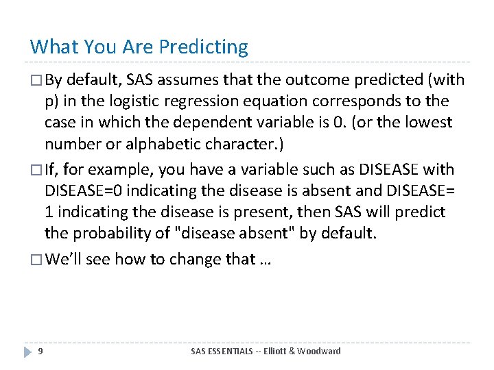
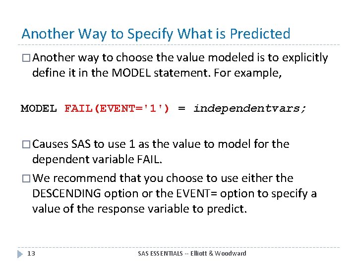
What You Are Predicting � By default, SAS assumes that the outcome predicted (with p) in the logistic regression equation corresponds to the case in which the dependent variable is 0. (or the lowest number or alphabetic character. ) � If, for example, you have a variable such as DISEASE with DISEASE=0 indicating the disease is absent and DISEASE= 1 indicating the disease is present, then SAS will predict the probability of "disease absent" by default. � We’ll see how to change that … 9 SAS ESSENTIALS -- Elliott & Woodward

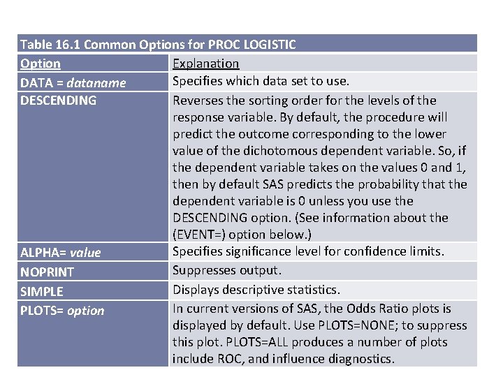
Table 16. 1 Common Options for PROC LOGISTIC Option Explanation Specifies which data set to use. DATA = dataname DESCENDING Reverses the sorting order for the levels of the response variable. By default, the procedure will predict the outcome corresponding to the lower value of the dichotomous dependent variable. So, if the dependent variable takes on the values 0 and 1, then by default SAS predicts the probability that the dependent variable is 0 unless you use the DESCENDING option. (See information about the (EVENT=) option below. ) Specifies significance level for confidence limits. ALPHA= value Suppresses output. NOPRINT Displays descriptive statistics. SIMPLE In current versions of SAS, the Odds Ratio plots is PLOTS= option displayed by default. Use PLOTS=NONE; to suppress this plot. PLOTS=ALL produces a number of plots 10 SAS ESSENTIALS -- Elliott & Woodward include ROC, and influence diagnostics.

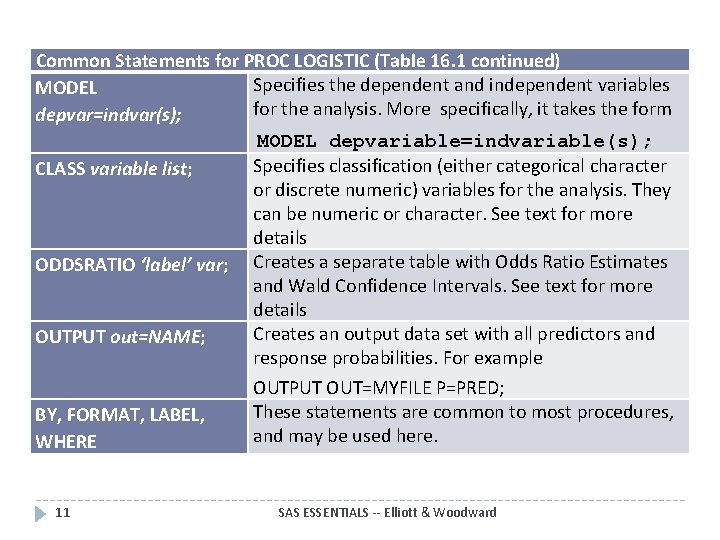
Common Statements for PROC LOGISTIC (Table 16. 1 continued) Specifies the dependent and independent variables MODEL for the analysis. More specifically, it takes the form depvar=indvar(s); MODEL depvariable=indvariable(s); Specifies classification (either categorical character CLASS variable list; or discrete numeric) variables for the analysis. They can be numeric or character. See text for more details ODDSRATIO ‘label’ var; Creates a separate table with Odds Ratio Estimates and Wald Confidence Intervals. See text for more details Creates an output data set with all predictors and OUTPUT out=NAME; response probabilities. For example OUTPUT OUT=MYFILE P=PRED; These statements are common to most procedures, BY, FORMAT, LABEL, and may be used here. WHERE 11 SAS ESSENTIALS -- Elliott & Woodward

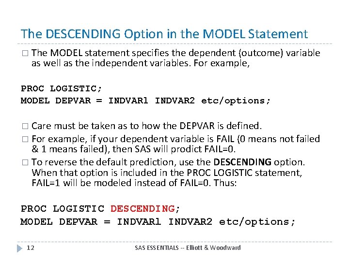
The DESCENDING Option in the MODEL Statement � The MODEL statement specifies the dependent (outcome) variable as well as the independent variables. For example, PROC LOGISTIC; MODEL DEPVAR = INDVARl INDVAR 2 etc/options; � Care must be taken as to how the DEPVAR is defined. � For example, if your dependent variable is FAIL (0 means not failed & 1 means failed), then SAS will prodict FAIL=0. � To reverse the default prediction, use the DESCENDING option. When that option is included in the PROC LOGISTIC statement, FAIL=1 will be modeled instead of FAIL=0. Thus: PROC LOGISTIC DESCENDING; MODEL DEPVAR = INDVARl INDVAR 2 etc/options; 12 SAS ESSENTIALS -- Elliott & Woodward

Another Way to Specify What is Predicted � Another way to choose the value modeled is to explicitly define it in the MODEL statement. For example, MODEL FAIL(EVENT='1') = independentvars; � Causes SAS to use 1 as the value to model for the dependent variable FAIL. � We recommend that you choose to use either the DESCENDING option or the EVENT= option to specify a value of the response variable to predict. 13 SAS ESSENTIALS -- Elliott & Woodward

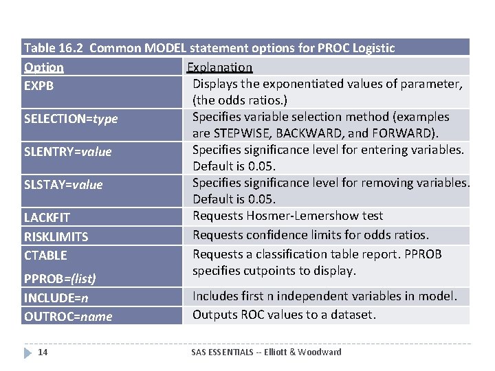
Table 16. 2 Common MODEL statement options for PROC Logistic Option Explanation Displays the exponentiated values of parameter, EXPB (the odds ratios. ) Specifies variable selection method (examples SELECTION=type are STEPWISE, BACKWARD, and FORWARD). Specifies significance level for entering variables. SLENTRY=value Default is 0. 05. Specifies significance level for removing variables. SLSTAY=value Default is 0. 05. Requests Hosmer-Lemershow test LACKFIT Requests confidence limits for odds ratios. RISKLIMITS Requests a classification table report. PPROB CTABLE specifies cutpoints to display. PPROB=(list) Includes first n independent variables in model. INCLUDE=n Outputs ROC values to a dataset. OUTROC=name 14 SAS ESSENTIALS -- Elliott & Woodward

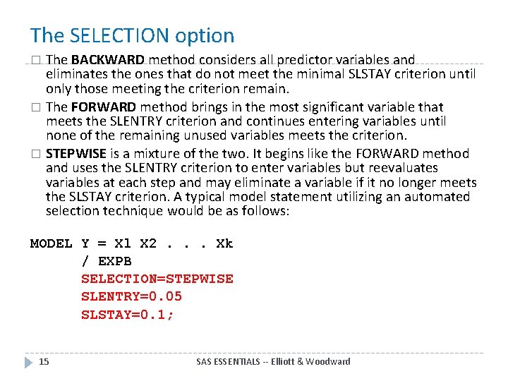
The SELECTION option The BACKWARD method considers all predictor variables and eliminates the ones that do not meet the minimal SLSTAY criterion until only those meeting the criterion remain. � The FORWARD method brings in the most significant variable that meets the SLENTRY criterion and continues entering variables until none of the remaining unused variables meets the criterion. � STEPWISE is a mixture of the two. It begins like the FORWARD method and uses the SLENTRY criterion to enter variables but reevaluates variables at each step and may eliminate a variable if it no longer meets the SLSTAY criterion. A typical model statement utilizing an automated selection technique would be as follows: � MODEL Y = Xl X 2. . . Xk / EXPB SELECTION=STEPWISE SLENTRY=0. 05 SLSTAY=0. 1; 15 SAS ESSENTIALS -- Elliott & Woodward

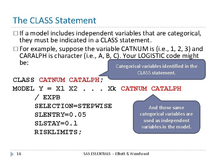
The CLASS Statement � If a model includes independent variables that are categorical, they must be indicated in a CLASS statement. � For example, suppose the variable CATNUM is (i. e. , 1, 2, 3) and CARALPH is character (i. e. , A, B, C). Your LOGISTIC code might be: Categorical variables identified in the CLASS statement. CLASS CATNUM CATALPH; MODEL Y = Xl X 2. . . Xk CATNUM CATALPH / EXPB SELECTION=STEPWISE And those same categorical variables are SLENTRY=0. 05 used as independent SLSTAY=0. l variables in the model. RISKLIMITS; 16 SAS ESSENTIALS -- Elliott & Woodward

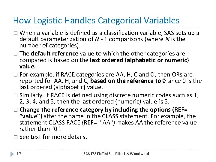
How Logistic Handles Categorical Variables � When a variable is defined as a classification variable, SAS sets up a default parameterization of N - 1 comparisons (where N is the number of categories). � The default reference value to which the other categories are compared is based on the last ordered (alphabetic or numeric) value. � For example, if RACE categories are AA, H, C and O, then ORs are reported for AA, H, and C, based on the reference to 0 since 0 is the last ordered (alphabetic) value. � Similarly, if RACE is defined using discrete numeric codes such as 1, 2, 3, 4, and 5, then the last ordered (numeric) value is 5. � Change the reference category by including the options (REF= "value") after the name in the CLASS statement. For example, the statement CLASS RACE (REF= " AA") makes AA the reference value rather than "0". � See text for more details. 17 SAS ESSENTIALS -- Elliott & Woodward

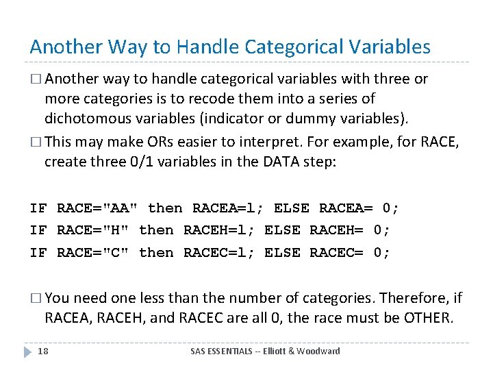
Another Way to Handle Categorical Variables � Another way to handle categorical variables with three or more categories is to recode them into a series of dichotomous variables (indicator or dummy variables). � This may make ORs easier to interpret. For example, for RACE, create three 0/1 variables in the DATA step: IF RACE="AA" then RACEA=l; ELSE RACEA= 0; IF RACE="H" then RACEH=l; ELSE RACEH= 0; IF RACE="C" then RACEC=l; ELSE RACEC= 0; � You need one less than the number of categories. Therefore, if RACEA, RACEH, and RACEC are all 0, the race must be OTHER. 18 SAS ESSENTIALS -- Elliott & Woodward

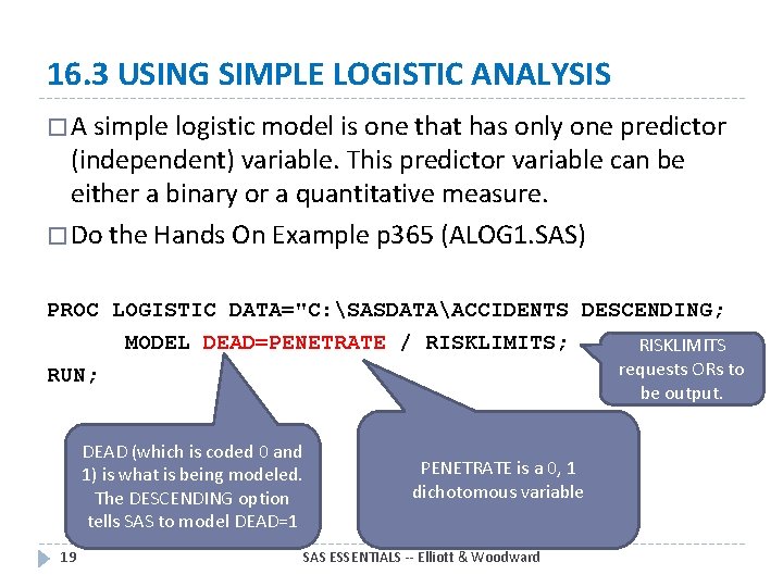
16. 3 USING SIMPLE LOGISTIC ANALYSIS � A simple logistic model is one that has only one predictor (independent) variable. This predictor variable can be either a binary or a quantitative measure. � Do the Hands On Example p 365 (ALOG 1. SAS) PROC LOGISTIC DATA="C: SASDATAACCIDENTS DESCENDING; MODEL DEAD=PENETRATE / RISKLIMITS; RISKLIMITS requests ORs to RUN; be output. DEAD (which is coded 0 and 1) is what is being modeled. The DESCENDING option tells SAS to model DEAD=1 19 PENETRATE is a 0, 1 dichotomous variable SAS ESSENTIALS -- Elliott & Woodward

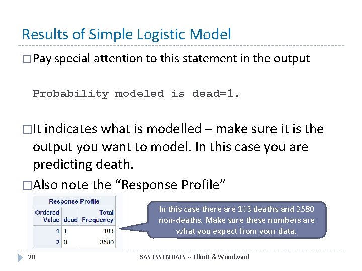
Results of Simple Logistic Model � Pay special attention to this statement in the output Probability modeled is dead=1. �It indicates what is modelled – make sure it is the output you want to model. In this case you are predicting death. �Also note the “Response Profile” In this case there are 103 deaths and 3580 non-deaths. Make sure these numbers are what you expect from your data. 20 SAS ESSENTIALS -- Elliott & Woodward

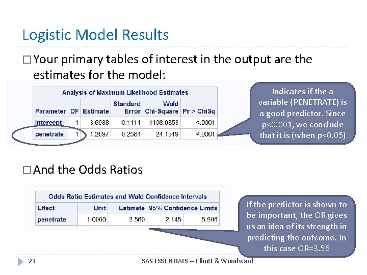
Logistic Model Results � Your primary tables of interest in the output are the estimates for the model: Indicates if the a variable (PENETRATE) is a good predictor. Since p<0. 001, we conclude that it is (when p<0. 05) � And the Odds Ratios If the predictor is shown to be important, the OR gives us an idea of its strength in predicting the outcome. In this case OR=3. 56 21 SAS ESSENTIALS -- Elliott & Woodward

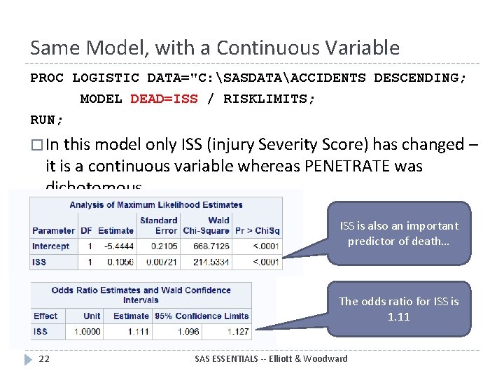
Same Model, with a Continuous Variable PROC LOGISTIC DATA="C: SASDATAACCIDENTS DESCENDING; MODEL DEAD=ISS / RISKLIMITS; RUN; � In this model only ISS (injury Severity Score) has changed – it is a continuous variable whereas PENETRATE was dichotomous. ISS is also an important predictor of death… The odds ratio for ISS is 1. 11 22 SAS ESSENTIALS -- Elliott & Woodward

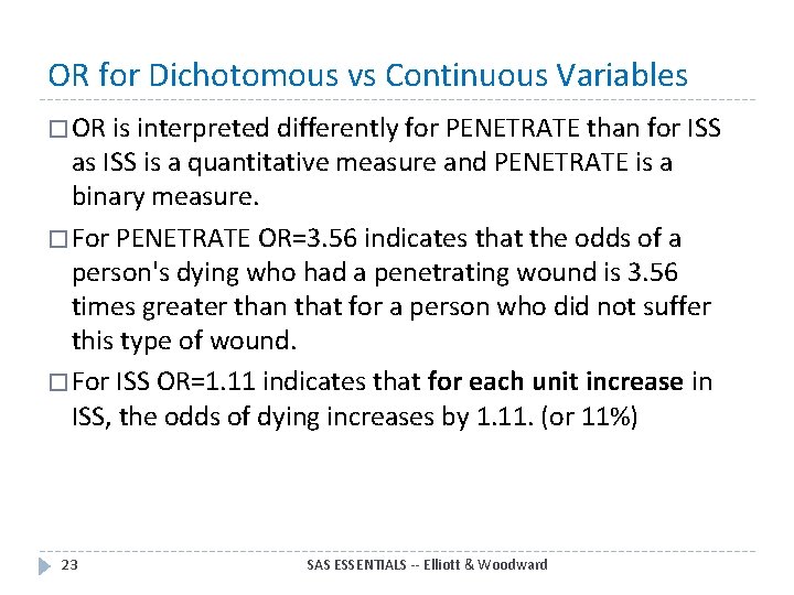
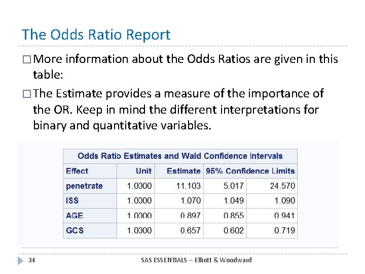
OR for Dichotomous vs Continuous Variables � OR is interpreted differently for PENETRATE than for ISS as ISS is a quantitative measure and PENETRATE is a binary measure. � For PENETRATE OR=3. 56 indicates that the odds of a person's dying who had a penetrating wound is 3. 56 times greater than that for a person who did not suffer this type of wound. � For ISS OR=1. 11 indicates that for each unit increase in ISS, the odds of dying increases by 1. 11. (or 11%) 23 SAS ESSENTIALS -- Elliott & Woodward

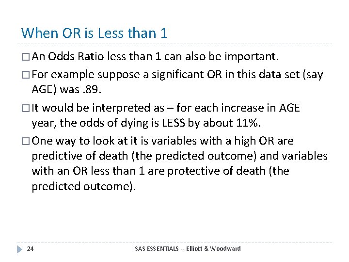
When OR is Less than 1 � An Odds Ratio less than 1 can also be important. � For example suppose a significant OR in this data set (say AGE) was. 89. � It would be interpreted as – for each increase in AGE year, the odds of dying is LESS by about 11%. � One way to look at it is variables with a high OR are predictive of death (the predicted outcome) and variables with an OR less than 1 are protective of death (the predicted outcome). 24 SAS ESSENTIALS -- Elliott & Woodward

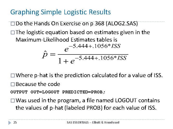
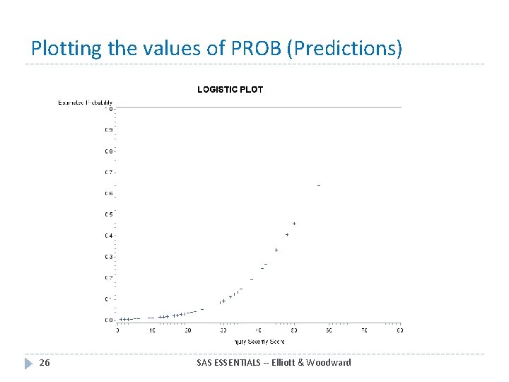
Graphing Simple Logistic Results � Do the Hands On Exercise on p 368 (ALOG 2. SAS) � The logistic equation based on estimates given in the Maximum-Likelihood Estimates tables is � Where p-hat is the prediction calculated for a value of ISS. � Because the code OUTPUT OUT=LOGOUT PREDICTED=PROB; � Was used in the program, a file named LOGOUT contains the values of p-hat (labeled PROB) for each value of ISS. 25 SAS ESSENTIALS -- Elliott & Woodward

Plotting the values of PROB (Predictions) 26 SAS ESSENTIALS -- Elliott & Woodward

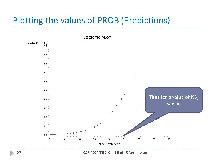
Plotting the values of PROB (Predictions) Thus for a value of ISS, say 50 27 SAS ESSENTIALS -- Elliott & Woodward

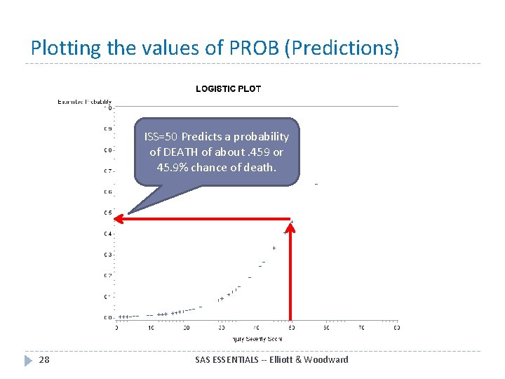
Plotting the values of PROB (Predictions) ISS=50 Predicts a probability of DEATH of about. 459 or 45. 9% chance of death. 28 SAS ESSENTIALS -- Elliott & Woodward

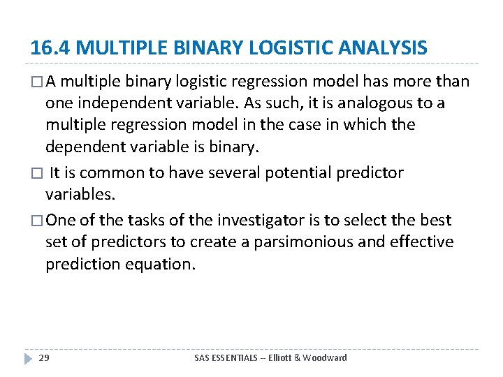
16. 4 MULTIPLE BINARY LOGISTIC ANALYSIS � A multiple binary logistic regression model has more than one independent variable. As such, it is analogous to a multiple regression model in the case in which the dependent variable is binary. � It is common to have several potential predictor variables. � One of the tasks of the investigator is to select the best set of predictors to create a parsimonious and effective prediction equation. 29 SAS ESSENTIALS -- Elliott & Woodward

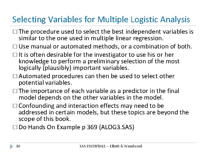
Selecting Variables for Multiple Logistic Analysis � The procedure used to select the best independent variables is similar to the one used in multiple linear regression. � Use manual or automated methods, or a combination of both. � It is often desirable for the investigator to use his or her knowledge to perform a preliminary selection of the most logically (plausibly) important variables. � Automated procedures can then be used to select other potential variables. � The importance of each variable as a predictor in the final model depends on the other variables in the model. � Confounding and interaction effects may need to be addressed in certain models, but these topics are beyond the scope of this book. � Do Hands On Example p 369 (ALOG 3. SAS) 30 SAS ESSENTIALS -- Elliott & Woodward

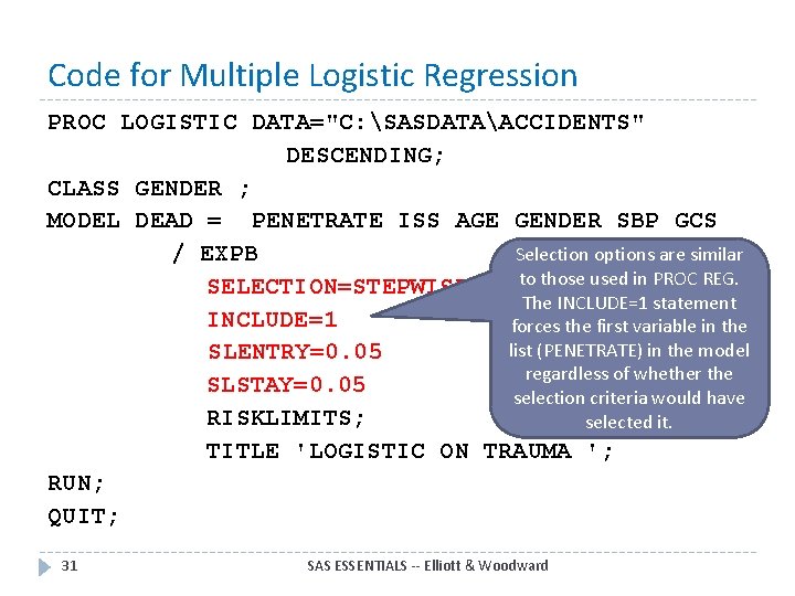
Code for Multiple Logistic Regression PROC LOGISTIC DATA="C: SASDATAACCIDENTS" DESCENDING; CLASS GENDER ; MODEL DEAD = PENETRATE ISS AGE GENDER SBP GCS / EXPB Selection options are similar to those used in PROC REG. SELECTION=STEPWISE The INCLUDE=1 statement INCLUDE=1 forces the first variable in the list (PENETRATE) in the model SLENTRY=0. 05 regardless of whether the SLSTAY=0. 05 selection criteria would have RISKLIMITS; selected it. TITLE 'LOGISTIC ON TRAUMA '; RUN; QUIT; 31 SAS ESSENTIALS -- Elliott & Woodward

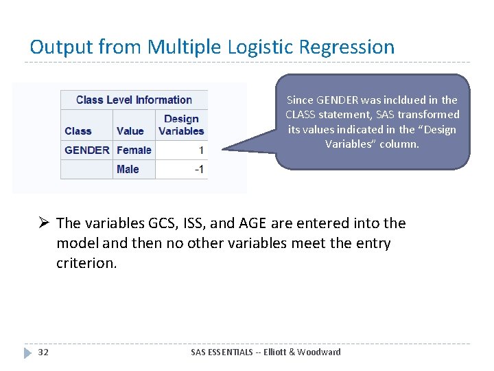
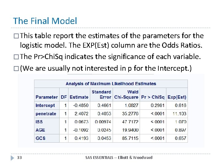
Output from Multiple Logistic Regression Since GENDER was incldued in the CLASS statement, SAS transformed its values indicated in the “Design Variables” column. Ø The variables GCS, ISS, and AGE are entered into the model and then no other variables meet the entry criterion. 32 SAS ESSENTIALS -- Elliott & Woodward

The Final Model � This table report the estimates of the parameters for the logistic model. The EXP(Est) column are the Odds Ratios. � The Pr>Chi. Sq indicates the significance of each variable. � (We are usually not interested in p for the Intercept. ) 33 SAS ESSENTIALS -- Elliott & Woodward

The Odds Ratio Report � More information about the Odds Ratios are given in this table: � The Estimate provides a measure of the importance of the OR. Keep in mind the different interpretations for binary and quantitative variables. 34 SAS ESSENTIALS -- Elliott & Woodward

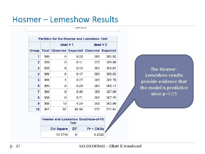
16. 5 GOING DEEPER: ASSESSING A MODEL'S FIT AND PREDICTIVE ABILITY � Once you decide on a final model, you should analyze that model for its predictive ability. � One method of analyzing the predictive capabilities of the logistic equation is to use the Hosmer and Lemeshow test. This test is based on dividing subjects into deciles on the basis of predicted probabilities � SAS reports chi-square statistics based on the observed and expected frequencies for subjects within these 10 categories. � A non-significant result is what you want – this provides evidence that the model is predictive. � Do the Hands On Exercise p 372 (ALOG 4. SAS) 35 SAS ESSENTIALS -- Elliott & Woodward

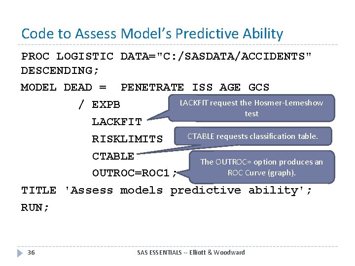
Code to Assess Model’s Predictive Ability PROC LOGISTIC DATA="C: /SASDATA/ACCIDENTS" DESCENDING; MODEL DEAD = PENETRATE ISS AGE GCS LACKFIT request the Hosmer-Lemeshow / EXPB test LACKFIT CTABLE requests classification table. RISKLIMITS CTABLE The OUTROC= option produces an ROC Curve (graph). OUTROC=ROC 1; TITLE 'Assess models predictive ability'; RUN; 36 SAS ESSENTIALS -- Elliott & Woodward

Hosmer – Lemeshow Results The Hosmer. Lemeshow results provide evidence that the model is predictive since p>0. 05 37 SAS ESSENTIALS -- Elliott & Woodward

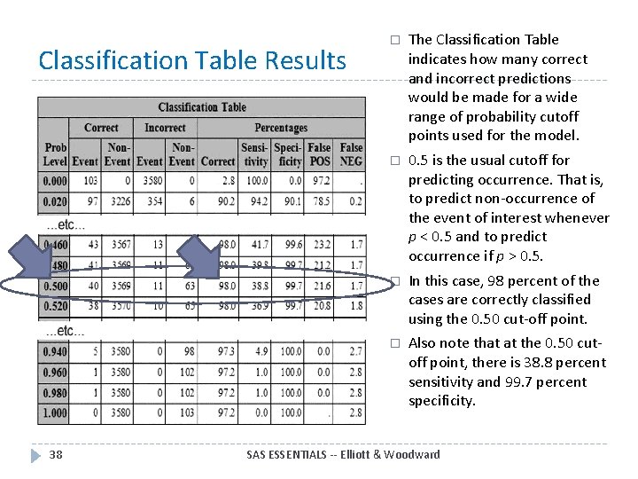
Classification Table Results 38 � The Classification Table indicates how many correct and incorrect predictions would be made for a wide range of probability cutoff points used for the model. � 0. 5 is the usual cutoff for predicting occurrence. That is, to predict non-occurrence of the event of interest whenever p < 0. 5 and to predict occurrence if p > 0. 5. � In this case, 98 percent of the cases are correctly classified using the 0. 50 cut-off point. � Also note that at the 0. 50 cutoff point, there is 38. 8 percent sensitivity and 99. 7 percent specificity. SAS ESSENTIALS -- Elliott & Woodward

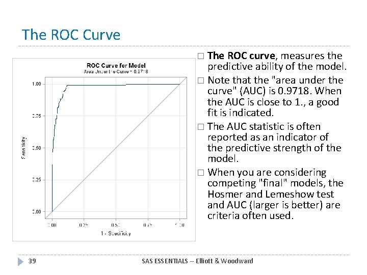
The ROC Curve � The ROC curve, measures the predictive ability of the model. � Note that the "area under the curve" (AUC) is 0. 9718. When the AUC is close to 1. , a good fit is indicated. � The AUC statistic is often reported as an indicator of the predictive strength of the model. � When you are considering competing "final" models, the Hosmer and Lemeshow test and AUC (larger is better) are criteria often used. 39 SAS ESSENTIALS -- Elliott & Woodward

16. 6 SUMMARY � This chapter provides examples of the use of SAS for running simple and multivariate logistic regression analyses. Also techniques for selecting a model and for assessing its predictive ability are illustrated. � Continue to Chapter 17: FACTOR ANALYSIS 40 SAS ESSENTIALS -- Elliott & Woodward

These slides are based on the book: Introduction to SAS Essentials Mastering SAS for Data Analytics, 2 nd Edition By Alan C, Elliott and Wayne A. Woodward Paperback: 512 pages Publisher: Wiley; 2 edition (August 3, 2015) Language: English ISBN-10: 111904216 X ISBN-13: 978 -1119042167 These slides are provided for you to use to teach SAS using this book. Feel free to modify them for your own needs. Please send comments about errors in the slides (or suggestions for improvements) to acelliott@smu. edu. Thanks. 41 SAS ESSENTIALS -- Elliott & Woodward