Introduction to Sampling based inference and MCMC Ata

Introduction to Sampling based inference and MCMC Ata Kaban School of Computer Science The University of Birmingham

The problem • Up till now we were trying to solve search problems (search for optima of functions, search for NN structures, search for solution to various problems) • Today we try to: – Compute volumes • Averages, expectations, integrals – Simulate a sample from a distribution of given shape • Some analogies with EA in that we work with ‘samples’ or ‘populations’

The Monte Carlo principle • p(x): a target density defined over a high-dimensional space (e. g. the space of all possible configurations of a system under study) • The idea of Monte Carlo techniques is to draw a set of (iid) samples {x 1, …, x. N} from p in order to approximate p with the empirical distribution • Using these samples we can approximate integrals I(f) (or v large sums) with tractable sums that converge (as the number of samples grows) to I(f)

Importance sampling • Target density p(x) known up to a constant • Task: compute Idea: • Introduce an arbitrary proposal density that includes the support of p. Then: – Sample from q instead of p – Weight the samples according to their ‘importance’ • It also implies that p(x) is approximated by Efficiency depends on a ‘good’ choice of q.

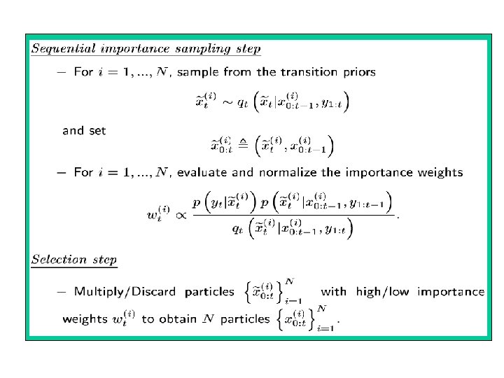
Sequential Monte Carlo • Sequential: – Real time processing – Dealing with non-stationarity – Not having to store the data • Goal: estimate the distrib of ‘hidden’ trajectories – We observe yt at each time t – We have a model: • Initial distribution: • Dynamic model: • Measurement model:

• Can define a proposal distribution: • Then the importance weights are: • Obs. Simplifying choice for proposal distribution: Then: ‘fitness’

‘proposed’ ‘weighted’ ‘re-sampled’ ----‘proposed’ ‘weighted’

Applications • Computer vision – Object tracking demo [Blake&Isard] • Speech & audio enhancement • Web statistics estimation • Regression & classification – Global maximization of MLPs [Freitas et al] • Bayesian networks – Details in Gilks et al book (in the School library) • Genetics & molecular biology • Robotics, etc.

M Isard & A Blake: CONDENSATION – conditional density propagation for visual tracking. J of Computer Vision, 1998

References & resources [1] M Isard & A Blake: CONDENSATION – conditional density propagation for visual tracking. J of Computer Vision, 1998 Associated demos & further papers: http: //www. robots. ox. ac. uk/~misard/condensation. html [2] C Andrieu, N de Freitas, A Doucet, M Jordan: An Introduction to MCMC for machine learning. Machine Learning, vol. 50, pp. 5 -43, Jan. - Feb. 2003. Nando de Freitas’ MCMC papers & sw http: //www. cs. ubc. ca/~nando/software. html [3] MCMC preprint service http: //www. statslab. cam. ac. uk/~mcmc/pages/links. html [4] W. R. Gilks, S. Richardson & D. J. Spiegelhalter: Markov Chain Monte Carlo in Practice. Chapman & Hall, 1996

The Markov Chain Monte Carlo (MCMC) idea • Design a Markov Chain on finite state space …such that when simulating a trajectory of states from it, it will explore the state space spending more time in the most important regions (i. e. where p(x) is large)

Stationary distribution of a MC • Supposing you browse this for infinitely long time, what is the probability to be at page x i. • No matter where you started off. =>Page. Rank (Google)

Google vs. MCMC • Google is given T and finds p(x) • MCMC is given p(x) and finds T – But it also needs a ‘proposal (transition) probability distribution’ to be specified. • Q: Do all MCs have a stationary distribution? • A: No.

Conditions for existence of a unique stationary distribution • Irreducibility – The transition graph is connected (any state can be reached) • Aperiodicity – State trajectories drawn from the transition don’t get trapped into cycles • MCMC samplers are irreducible and aperiodic MCs that converge to the target distribution • These 2 conditions are not easy to impose directly

Reversibility • Reversibility (also called ‘detailed balance’) is a sufficient (but not necessary) condition for p(x) to be the stationary distribution. • It is easier to work with this condition.

MCMC algorithms • Metropolis-Hastings algorithm • Metropolis algorithm – Mixtures and blocks • Gibbs sampling • other • Sequential Monte Carlo & Particle Filters

The Metropolis-Hastings and the Metropolis algorithm as a special case Obs. The target distrib p(x) in only needed up to normalisation.

Examples of M-H simulations with q a Gaussian with variance sigma

Variations on M-H: Using mixtures and blocks • Mixtures (eg. of global & local distributions) – MC 1 with T 1 and having p(x) as stationary p – MC 2 with T 2 also having p(x) as stationary p – New MCs can be obtained: T 1*T 2, or a*T 1 + (1 -a)*T 2, which also have p(x) • Blocks – Split the multivariate state vector into blocks or components, that can be updated separately – Tradeoff: small blocks – slow exploration of target p large blocks – low accept rate

Gibbs sampling • Component-wise proposal q: Where the notation means: • Homework: Show that in this case, the acceptance probability is =1 [see [2], pp. 21]

Gibbs sampling algorithm

More advanced sampling techniques • Auxiliary variable samplers – Hybrid Monte Carlo • Uses the gradient of p – Tries to avoid ‘random walk’ behavior, i. e. to speed up convergence • Reversible jump MCMC – For comparing models of different dimensionalities (in ‘model selection’ problems) • Adaptive MCMC – Trying to automate the choice of q