Introduction to ROC curves ROC Receiver Operating Characteristic

Introduction to ROC curves ● ROC = Receiver Operating Characteristic ● Started in electronic signal detection theory (1940 s - 1950 s) ● Has become very popular in biomedical applications, particularly radiology and imaging ● גם בשימוש בכריית מידע

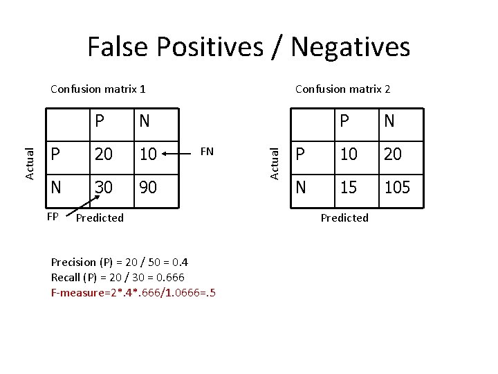
Confusion matrix 1 Confusion matrix 2 P N P 20 10 P 10 20 N 30 90 N 15 105 FP FN Predicted Precision (P) = 20 / 50 = 0. 4 Recall (P) = 20 / 30 = 0. 666 F-measure=2*. 4*. 666/1. 0666=. 5 Actual False Positives / Negatives Predicted

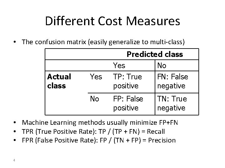
Different Cost Measures • The confusion matrix (easily generalize to multi-class) Actual class Yes No Predicted class Yes No TP: True FN: False positive negative FP: False positive TN: True negative • Machine Learning methods usually minimize FP+FN • TPR (True Positive Rate): TP / (TP + FN) = Recall • FPR (False Positive Rate): FP / (TN + FP) = Precision 4

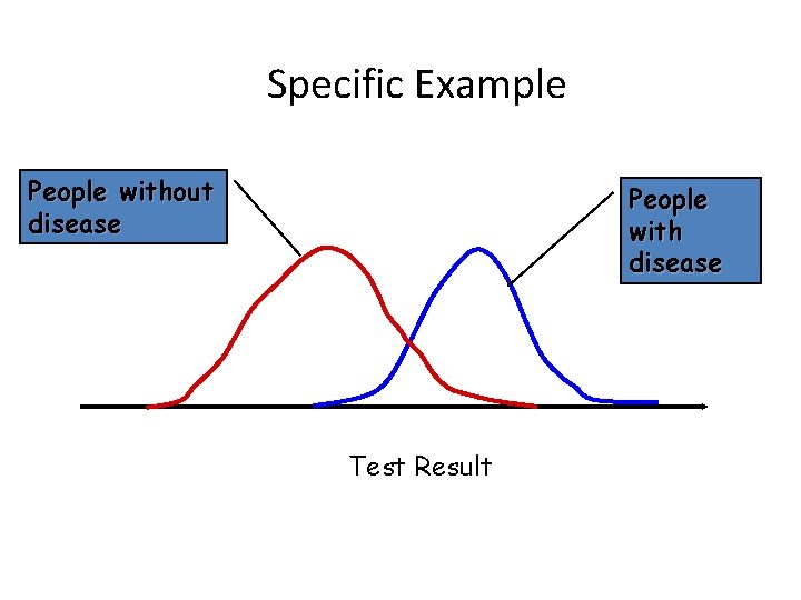
Specific Example People without disease People with disease Test Result

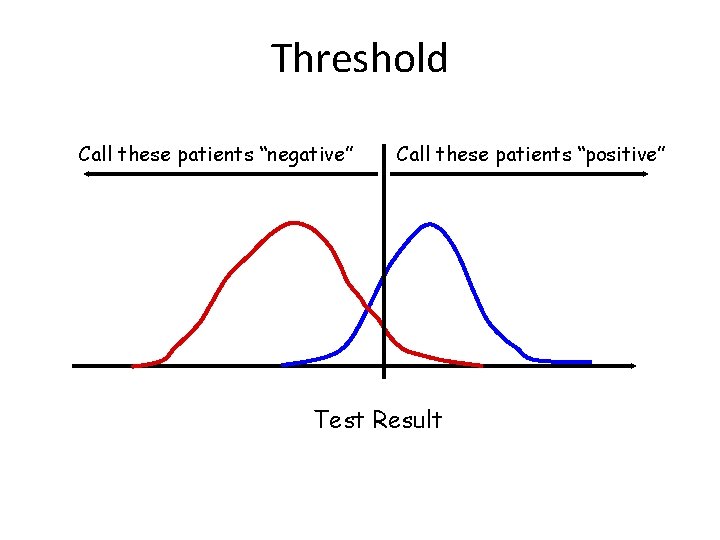
Threshold Call these patients “negative” Call these patients “positive” Test Result

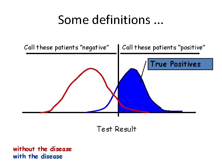
Some definitions. . . Call these patients “negative” Call these patients “positive” True Positives Test Result without the disease with the disease

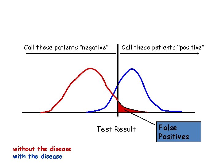
Call these patients “negative” Call these patients “positive” Test Result without the disease with the disease False Positives

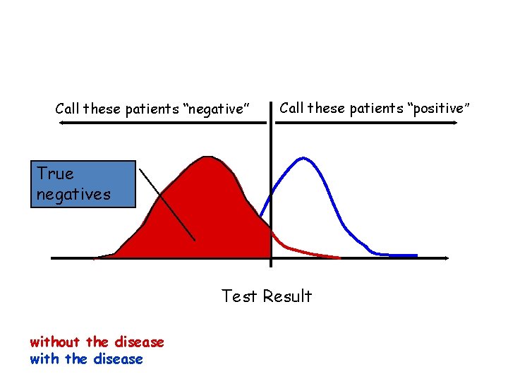
Call these patients “negative” Call these patients “positive” True negatives Test Result without the disease with the disease

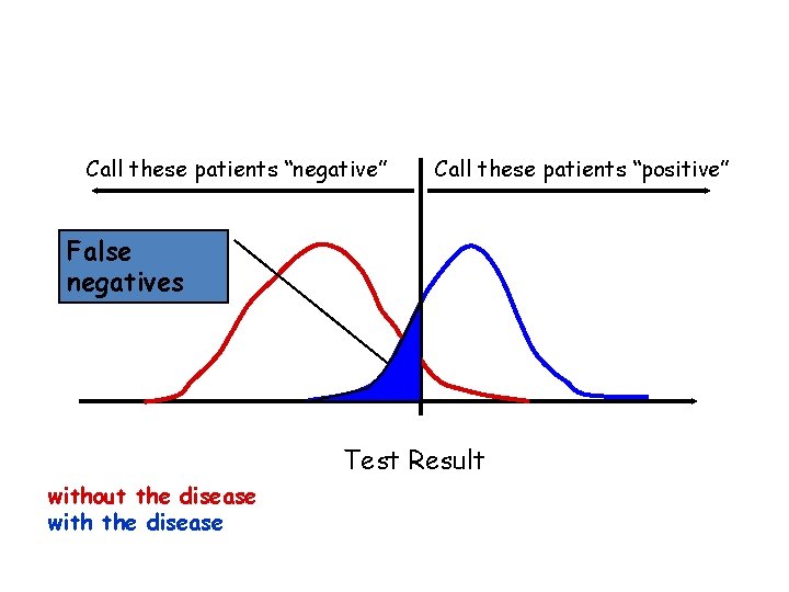
Call these patients “negative” Call these patients “positive” False negatives Test Result without the disease with the disease

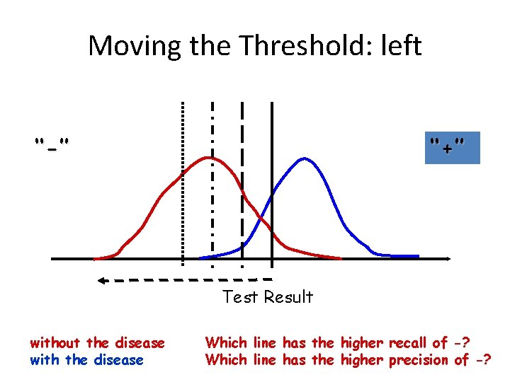
Moving the Threshold: left ‘‘-’’ ‘‘+’’ Test Result without the disease with the disease Which line has the higher recall of -? Which line has the higher precision of -?

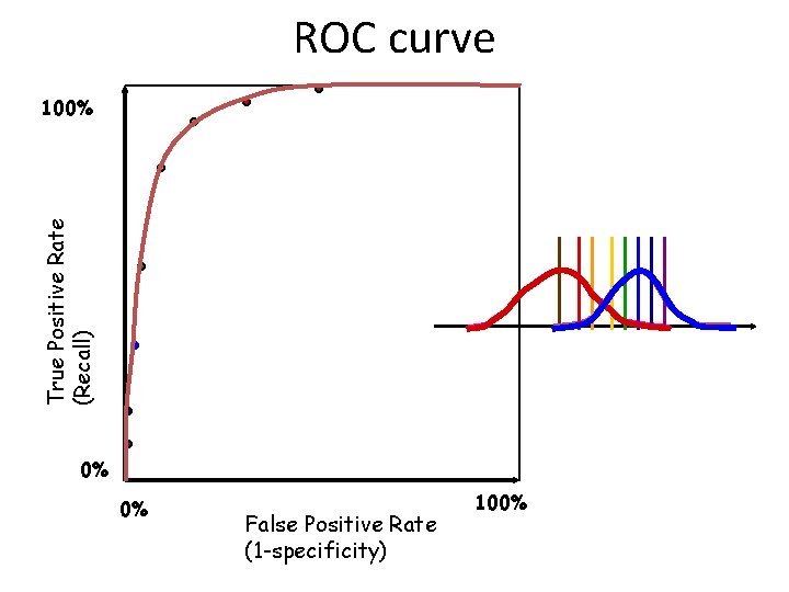
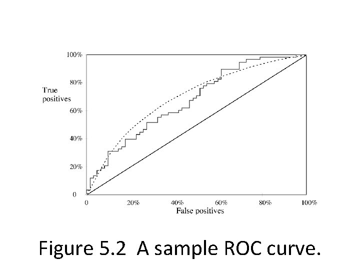
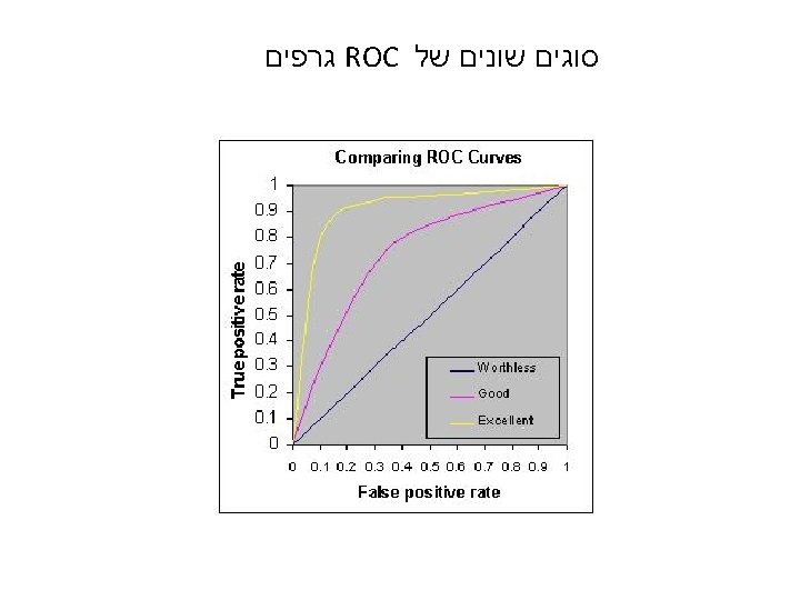
ROC curve True Positive Rate (Recall) 100% 0% 0% False Positive Rate (1 -specificity) 100%

Figure 5. 2 A sample ROC curve.

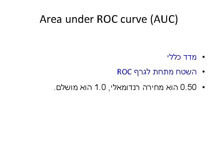
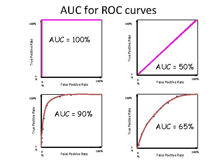
AUC for ROC curves 100% True Positive Rate AUC = 100% AUC = 50% 0 % 0 % False Positive Rate 100% True Positive Rate 100% 0 % AUC = 90% 0 % False Positive Rate 100% 0 % AUC = 65% 0 % False Positive Rate 100%

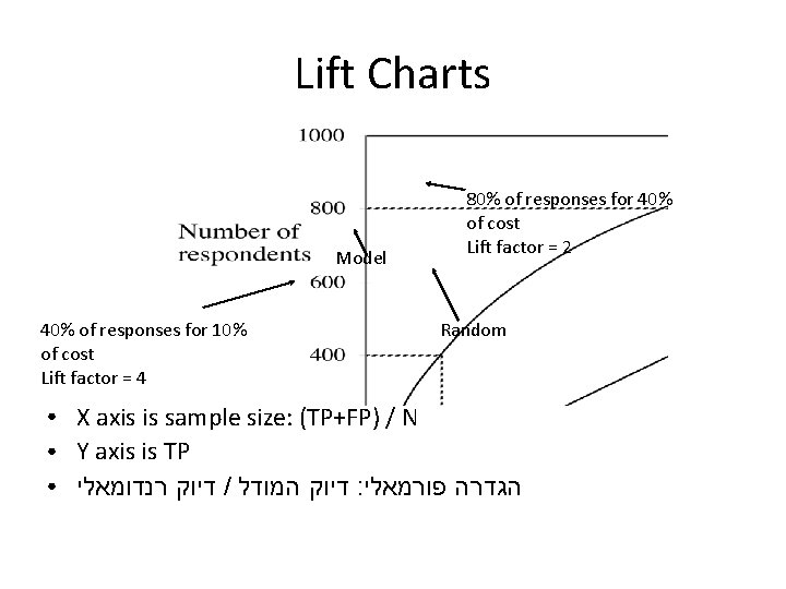
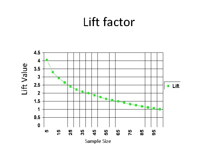
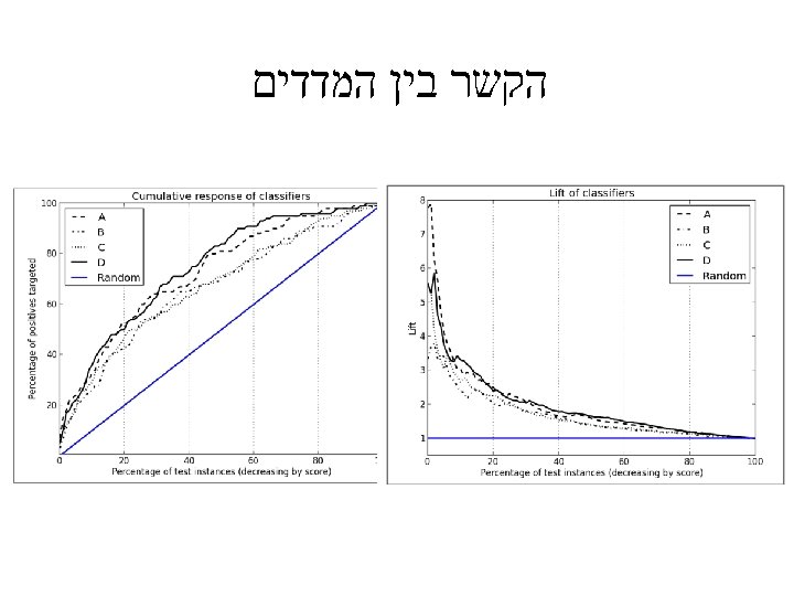
Lift Charts Model 40% of responses for 10% of cost Lift factor = 4 ● ● ● 80% of responses for 40% of cost Lift factor = 2 Random X axis is sample size: (TP+FP) / N Y axis is TP דיוק רנדומאלי / דיוק המודל : הגדרה פורמאלי

Lift Value Lift factor Sample Size

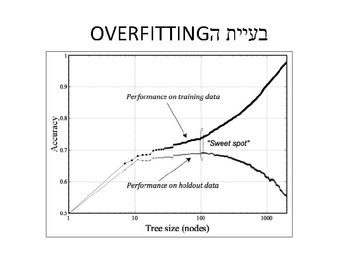
OVERFITTING בעיית ה

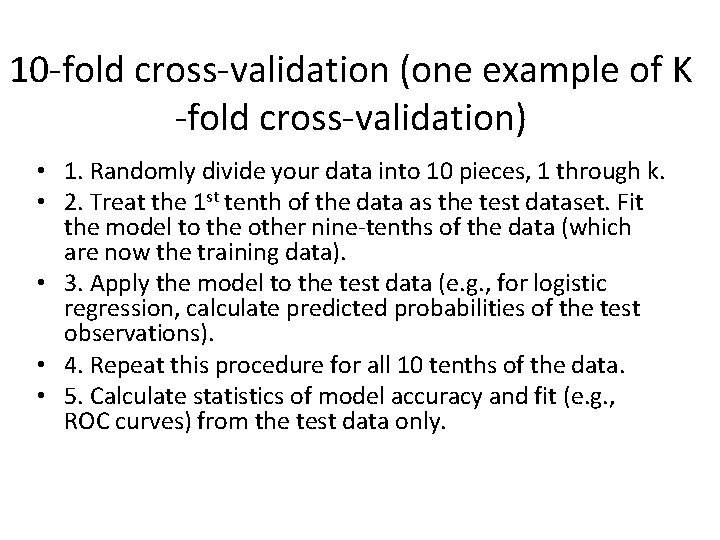
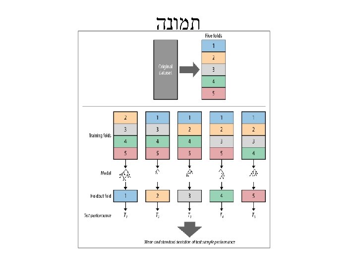
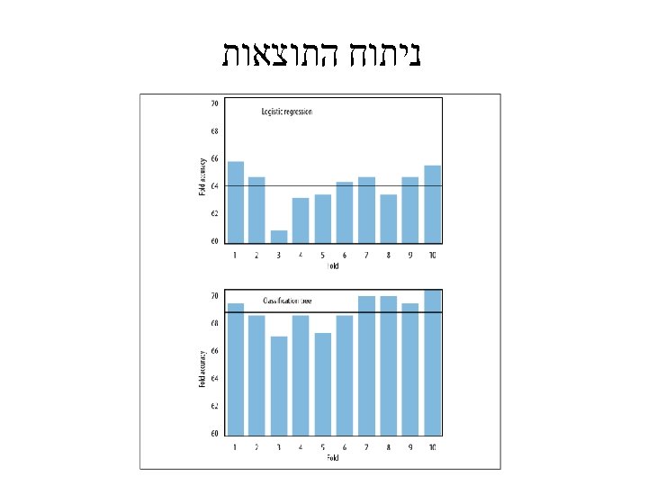
10 -fold cross-validation (one example of K -fold cross-validation) • 1. Randomly divide your data into 10 pieces, 1 through k. • 2. Treat the 1 st tenth of the data as the test dataset. Fit the model to the other nine-tenths of the data (which are now the training data). • 3. Apply the model to the test data (e. g. , for logistic regression, calculate predicted probabilities of the test observations). • 4. Repeat this procedure for all 10 tenths of the data. • 5. Calculate statistics of model accuracy and fit (e. g. , ROC curves) from the test data only.

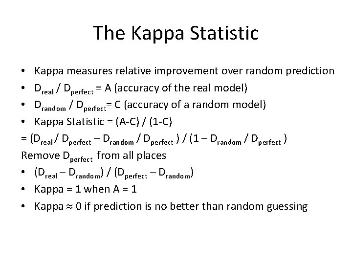
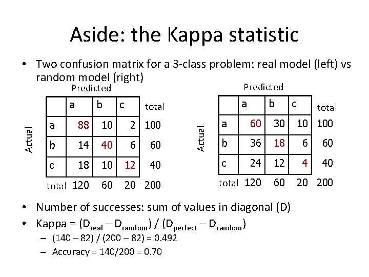
The Kappa Statistic • Kappa measures relative improvement over random prediction • Dreal / Dperfect = A (accuracy of the real model) • Drandom / Dperfect= C (accuracy of a random model) • Kappa Statistic = (A-C) / (1 -C) = (Dreal / Dperfect – Drandom / Dperfect ) / (1 – Drandom / Dperfect ) Remove Dperfect from all places • (Dreal – Drandom) / (Dperfect – Drandom) • Kappa = 1 when A = 1 • Kappa 0 if prediction is no better than random guessing

Aside: the Kappa statistic • Two confusion matrix for a 3 -class problem: real model (left) vs random model (right) Predicted b c a total a 88 10 2 100 b 14 40 6 60 c 18 10 12 40 total 120 60 20 200 Actual a b total a 60 30 b 36 18 6 60 c 24 12 4 40 total 120 60 • Number of successes: sum of values in diagonal (D) • Kappa = (Dreal – Drandom) / (Dperfect – Drandom) – (140 – 82) / (200 – 82) = 0. 492 – Accuracy = 140/200 = 0. 70 c 10 100 20 200

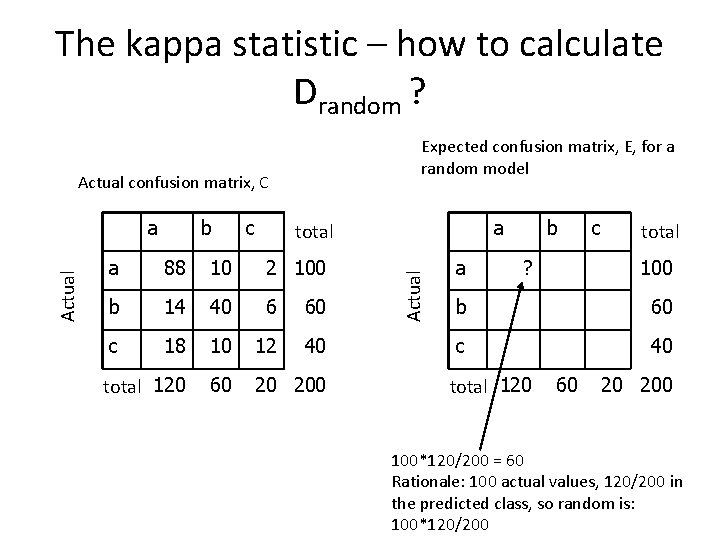
The kappa statistic – how to calculate Drandom ? Expected confusion matrix, E, for a random model Actual confusion matrix, C b c a total a 88 10 2 100 b 14 40 6 60 c 18 10 12 40 total 120 60 20 200 Actual a a b ? c total 100 b 60 c 40 total 120 60 20 200 100*120/200 = 60 Rationale: 100 actual values, 120/200 in the predicted class, so random is: 100*120/200