Introduction to RNASeq Describe assay data produced Describe

Introduction to RNA-Seq • Describe assay & data produced • Describe differential expression analysis process • Describe confirmation/validation process – Check gene expression graphs in Genome Browser 1

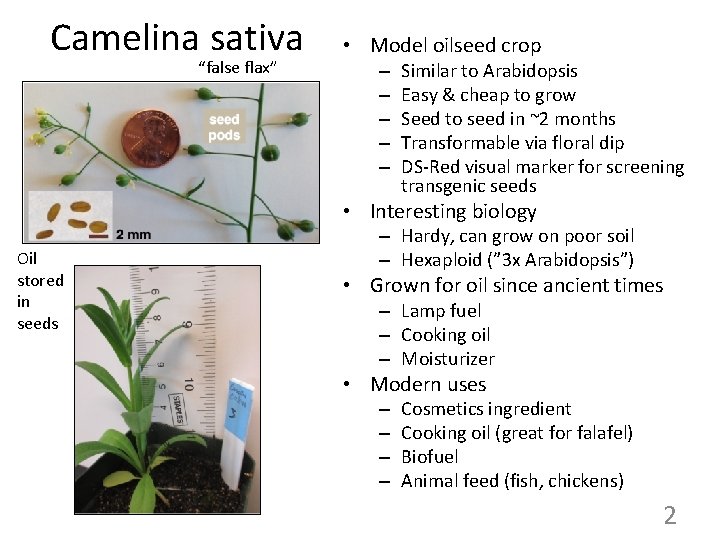
Camelina sativa “false flax” • Model oilseed crop – – – Similar to Arabidopsis Easy & cheap to grow Seed to seed in ~2 months Transformable via floral dip DS-Red visual marker for screening transgenic seeds • Interesting biology Oil stored in seeds – Hardy, can grow on poor soil – Hexaploid (” 3 x Arabidopsis”) • Grown for oil since ancient times – Lamp fuel – Cooking oil – Moisturizer • Modern uses – – Cosmetics ingredient Cooking oil (great for falafel) Biofuel Animal feed (fish, chickens) 2

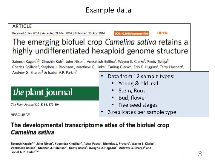
Example data • Data from 12 sample types: • Young & old leaf • Stem, Root • Bud, flower • Five seed stages • 3 replicates per sample type 3

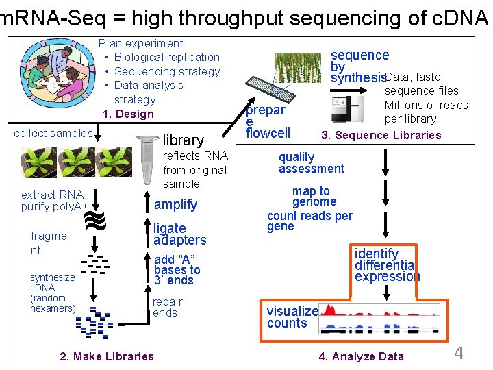
m. RNA-Seq = high throughput sequencing of c. DNA Plan experiment • Biological replication • Sequencing strategy • Data analysis strategy 1. Design collect samples extract RNA, purify poly. A+ ~ ~ fragme nt -----synthesize c. DNA (random hexamers) -- ------ library reflects RNA from original sample amplify ligate adapters sequence by synthesis. Data, fastq sequence files Millions of reads per library 3. Sequence Libraries prepar e flowcell quality assessment map to genome count reads per gene identify differential expression add “A” bases to 3’ ends repair ends 2. Make Libraries visualize counts 4. Analyze Data 4

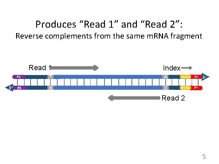
Produces “Read 1” and “Read 2”: Reverse complements from the same m. RNA fragment Read 1 Index Read 2 5

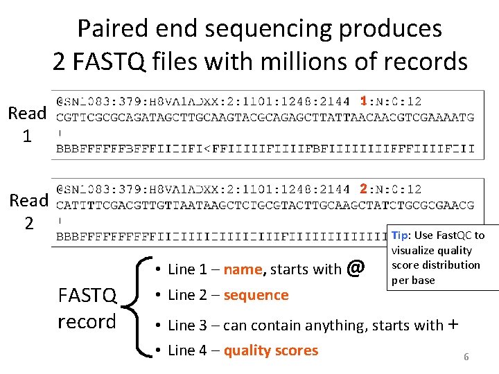
Paired end sequencing produces 2 FASTQ files with millions of records Read 1 1 Read 2 2 FASTQ record • Line 1 – name, starts with @ • Line 2 – sequence Tip: Use Fast. QC to visualize quality score distribution per base • Line 3 – can contain anything, starts with + • Line 4 – quality scores 6

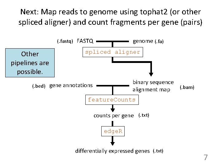
Next: Map reads to genome using tophat 2 (or other spliced aligner) and count fragments per gene (pairs) genome (. fa) (. fastq) FASTQ Other pipelines are possible. spliced aligner binary sequence alignment map (. bed) gene annotations (. bam) feature. Counts counts per gene (. txt) edge. R differentially expressed genes (. txt) 7

Introduction to RNA-Seq • Describe assay & data produced • Describe differential expression analysis process • Describe confirmation/validation process – Check gene expression graphs in Genome Browser 8

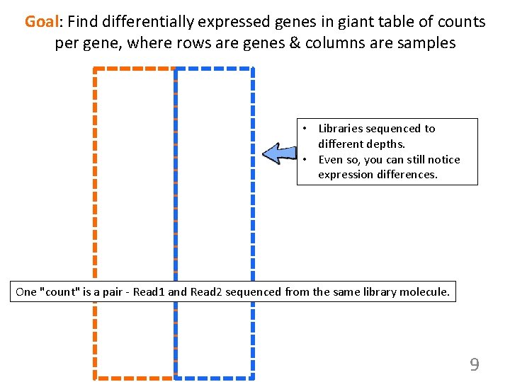
Goal: Find differentially expressed genes in giant table of counts per gene, where rows are genes & columns are samples • Libraries sequenced to different depths. • Even so, you can still notice expression differences. One "count" is a pair - Read 1 and Read 2 sequenced from the same library molecule. 9

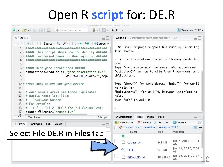
Open R script for: DE. R Select File DE. R in Files tab 10

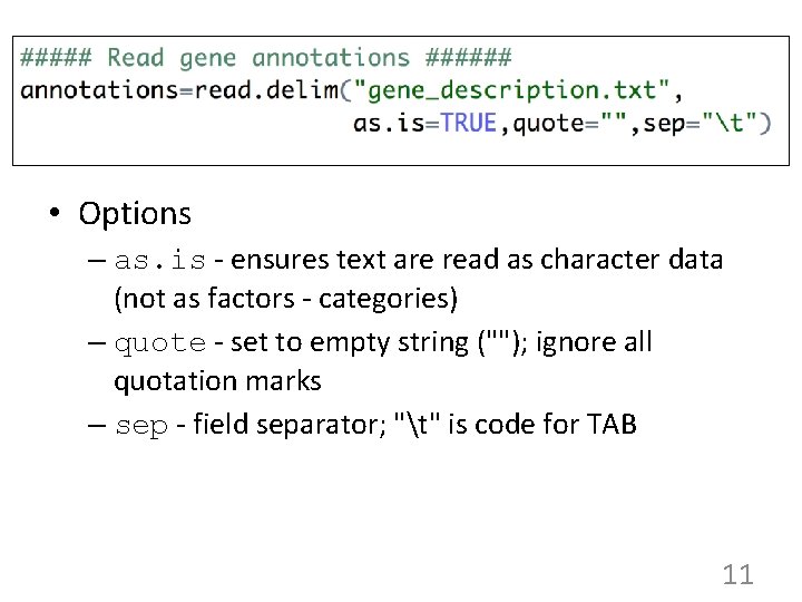
• Options – as. is - ensures text are read as character data (not as factors - categories) – quote - set to empty string (""); ignore all quotation marks – sep - field separator; "t" is code for TAB 11

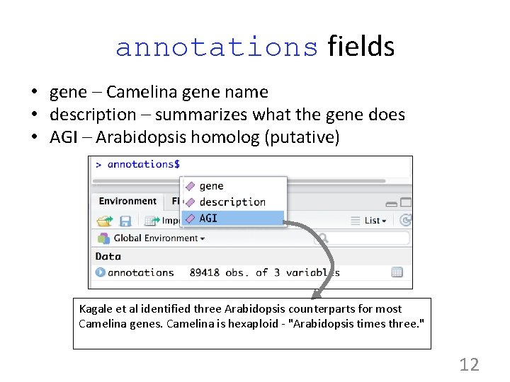
annotations fields • gene – Camelina gene name • description – summarizes what the gene does • AGI – Arabidopsis homolog (putative) Kagale et al identified three Arabidopsis counterparts for most Camelina genes. Camelina is hexaploid - "Arabidopsis times three. " 12

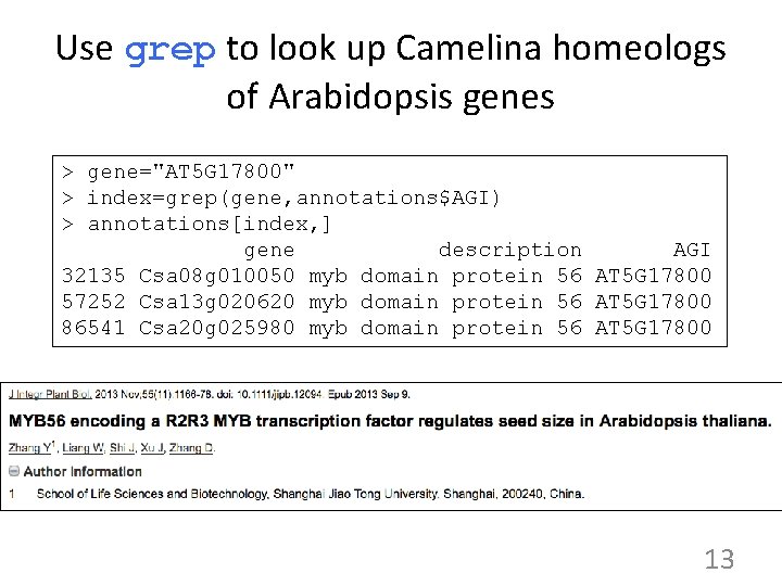
Use grep to look up Camelina homeologs of Arabidopsis genes > gene="AT 5 G 17800" > index=grep(gene, annotations$AGI) > annotations[index, ] gene description AGI 32135 Csa 08 g 010050 myb domain protein 56 AT 5 G 17800 57252 Csa 13 g 020620 myb domain protein 56 AT 5 G 17800 86541 Csa 20 g 025980 myb domain protein 56 AT 5 G 17800 13

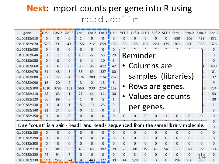
Next: Import counts per gene into R using read. delim Reminder: • Columns are samples (libraries) • Rows are genes. • Values are counts per genes. One "count" is a pair - Read 1 and Read 2 sequenced from the same library molecule. 14

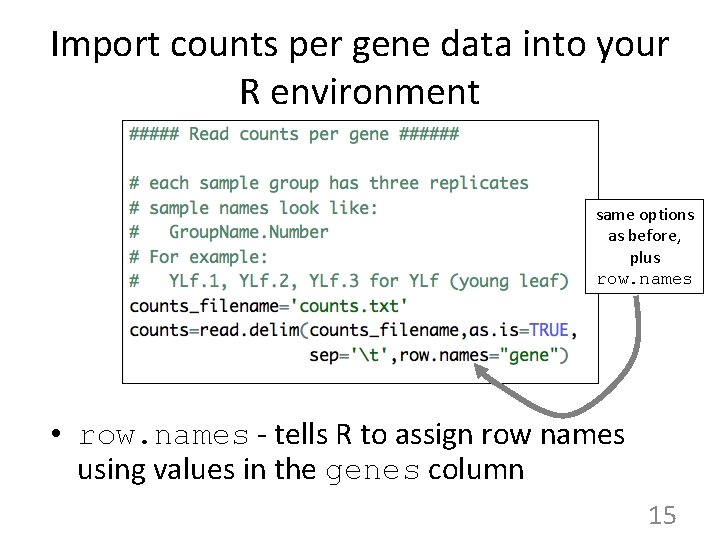
Import counts per gene data into your R environment same options as before, plus row. names • row. names - tells R to assign row names using values in the genes column 15

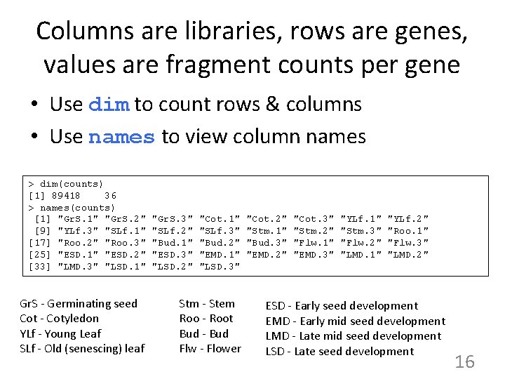
Columns are libraries, rows are genes, values are fragment counts per gene • Use dim to count rows & columns • Use names to view column names > dim(counts) [1] 89418 36 > names(counts) [1] "Gr. S. 1" "Gr. S. 2" [9] "YLf. 3" "SLf. 1" [17] "Roo. 2" "Roo. 3" [25] "ESD. 1" "ESD. 2" [33] "LMD. 3" "LSD. 1" Gr. S - Germinating seed Cot - Cotyledon YLf - Young Leaf SLf - Old (senescing) leaf "Gr. S. 3" "SLf. 2" "Bud. 1" "ESD. 3" "LSD. 2" "Cot. 1" "SLf. 3" "Bud. 2" "EMD. 1" "LSD. 3" Stm - Stem Roo - Root Bud - Bud Flw - Flower "Cot. 2" "Stm. 1" "Bud. 3" "EMD. 2" "Cot. 3" "Stm. 2" "Flw. 1" "EMD. 3" "YLf. 1" "Stm. 3" "Flw. 2" "LMD. 1" "YLf. 2" "Roo. 1" "Flw. 3" "LMD. 2" ESD - Early seed development EMD - Early mid seed development LMD - Late mid seed development LSD - Late seed development 16

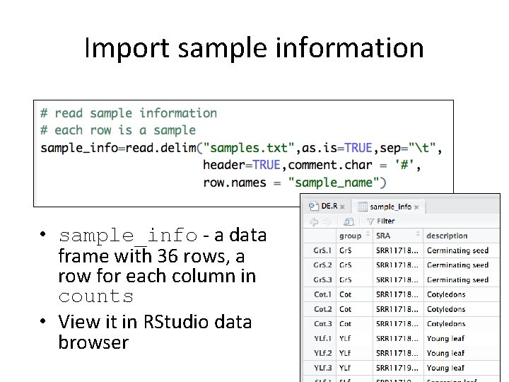
Import sample information • sample_info - a data frame with 36 rows, a row for each column in counts • View it in RStudio data browser 17

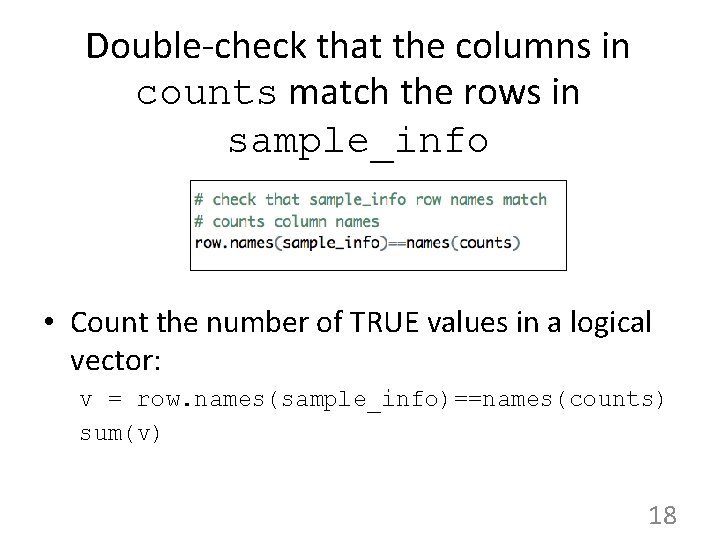
Double-check that the columns in counts match the rows in sample_info • Count the number of TRUE values in a logical vector: v = row. names(sample_info)==names(counts) sum(v) 18

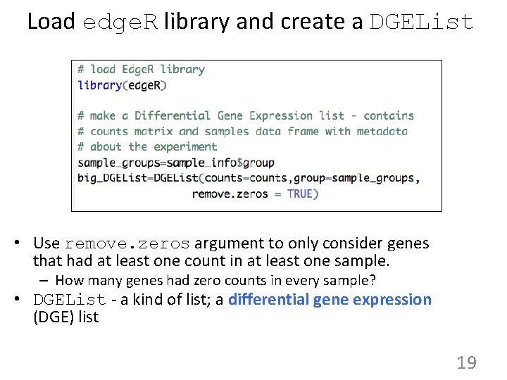
Load edge. R library and create a DGEList • Use remove. zeros argument to only consider genes that had at least one count in at least one sample. – How many genes had zero counts in every sample? • DGEList - a kind of list; a differential gene expression (DGE) list 19

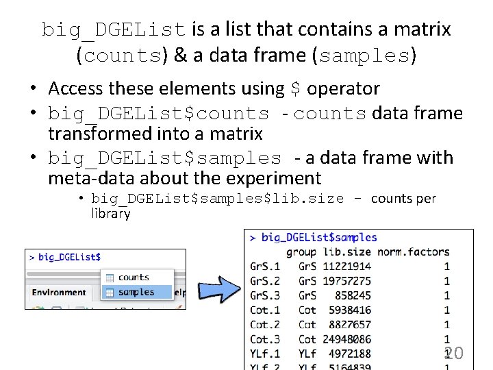
big_DGEList is a list that contains a matrix (counts) & a data frame (samples) • Access these elements using $ operator • big_DGEList$counts - counts data frame transformed into a matrix • big_DGEList$samples - a data frame with meta-data about the experiment • big_DGEList$samples$lib. size - counts per library 20

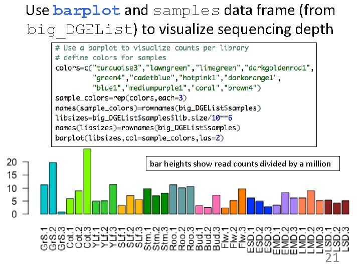
Use barplot and samples data frame (from big_DGEList) to visualize sequencing depth bar heights show read counts divided by a million 21

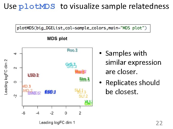
Use plot. MDS to visualize sample relatedness • Samples with similar expression are closer. • Replicates should be closest. 22

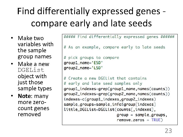
Find differentially expressed genes compare early and late seeds • Make two variables with the sample group names • Make a new DGEList object with just those sample types • Note: many more zerocount genes removed 23

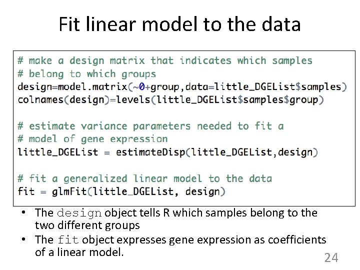
Fit linear model to the data • The design object tells R which samples belong to the two different groups • The fit object expresses gene expression as coefficients of a linear model. 24

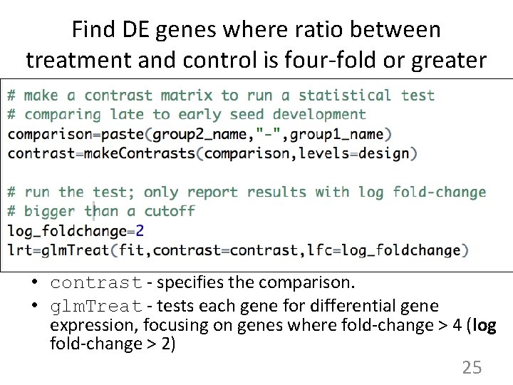
Find DE genes where ratio between treatment and control is four-fold or greater • contrast - specifies the comparison. • glm. Treat - tests each gene for differential gene expression, focusing on genes where fold-change > 4 (log fold-change > 2) 25

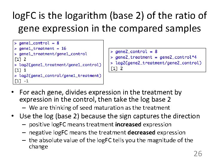
log. FC is the logarithm (base 2) of the ratio of gene expression in the compared samples • For each gene, divides expression in the treatment by expression in the control, then take the log base 2 – We are thinking of seed maturation as the treatment • Use the log (base 2) because the sign captures the direction – positive log. FC means treatment increased expression – negative log. FC means the treatment decreased expression – the absolute value of the log. FC tells you the magnitude of the change 26

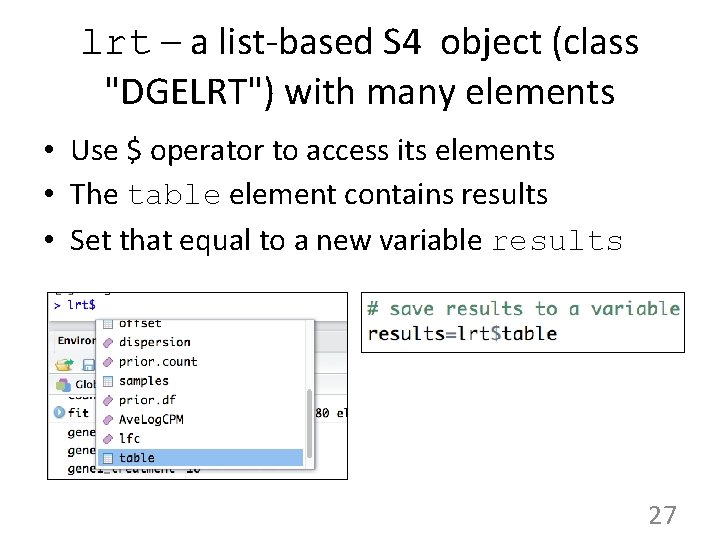
lrt – a list-based S 4 object (class "DGELRT") with many elements • Use $ operator to access its elements • The table element contains results • Set that equal to a new variable results 27

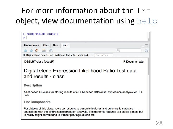
For more information about the lrt object, view documentation using help 28

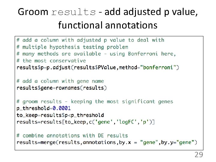
Groom results - add adjusted p value, functional annotations 29

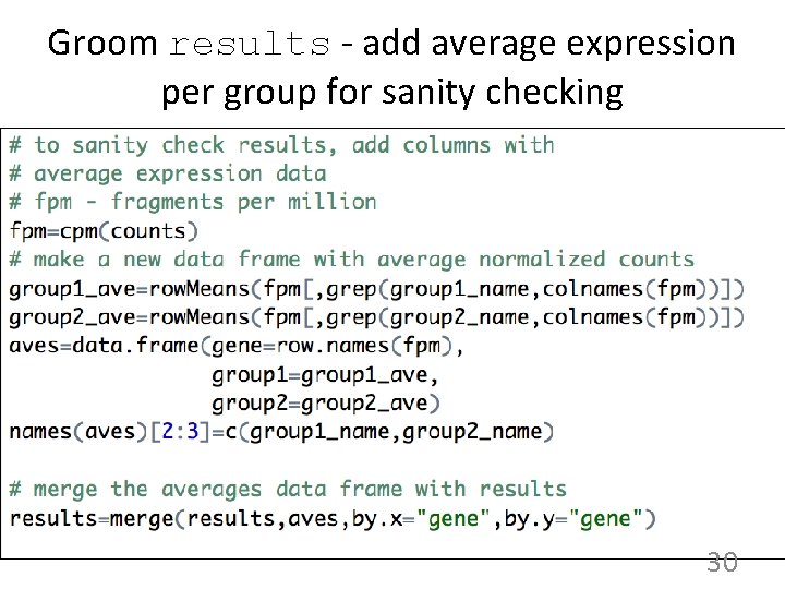
Groom results - add average expression per group for sanity checking 30

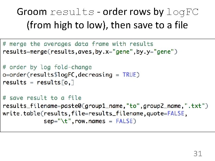
Groom results - order rows by log. FC (from high to low), then save to a file 31

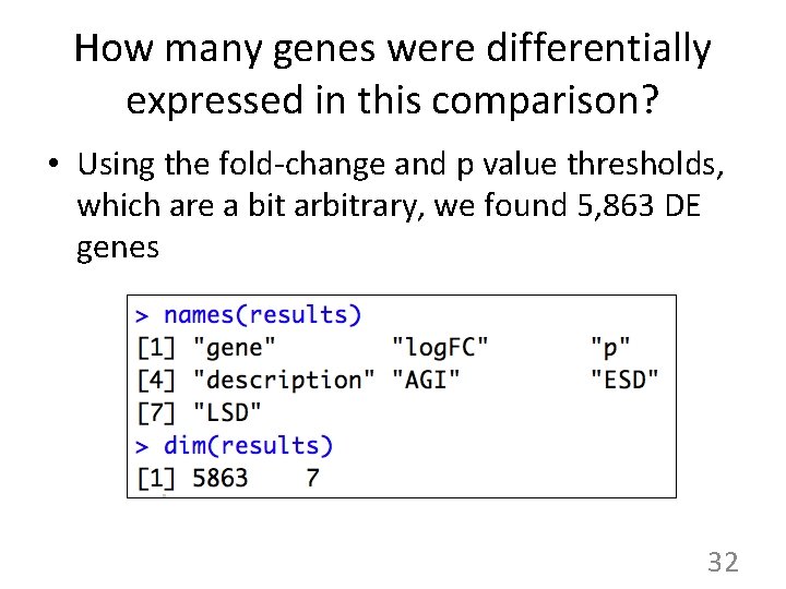
How many genes were differentially expressed in this comparison? • Using the fold-change and p value thresholds, which are a bit arbitrary, we found 5, 863 DE genes 32

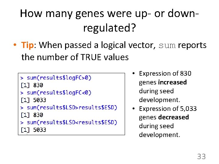
How many genes were up- or downregulated? • Tip: When passed a logical vector, sum reports the number of TRUE values • Expression of 830 genes increased during seed development. • Expression of 5, 033 genes decreased during seed development. 33

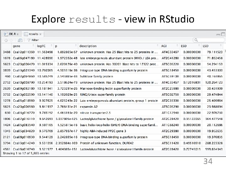
Explore results - view in RStudio 34

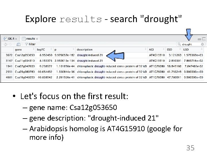
Explore results - search "drought" • Let's focus on the first result: – gene name: Csa 12 g 053650 – gene description: "drought-induced 21" – Arabidopsis homolog is AT 4 G 15910 (google for more info) 35

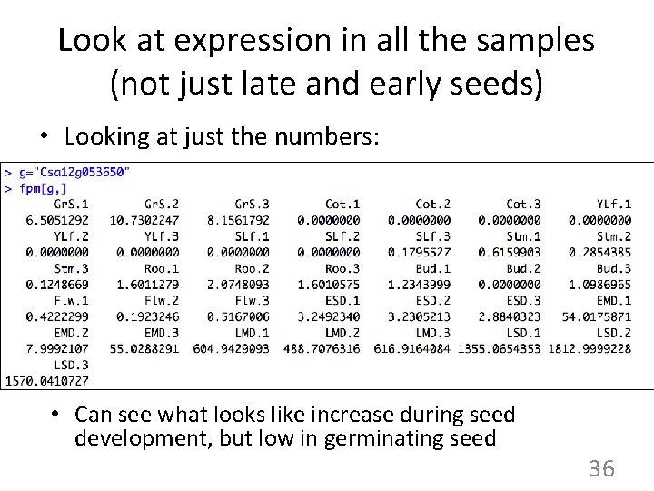
Look at expression in all the samples (not just late and early seeds) • Looking at just the numbers: • Can see what looks like increase during seed development, but low in germinating seed 36

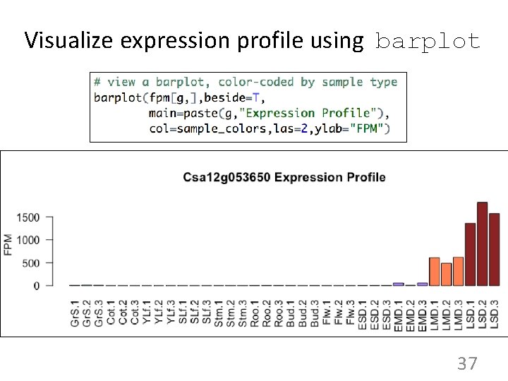
Visualize expression profile using barplot 37

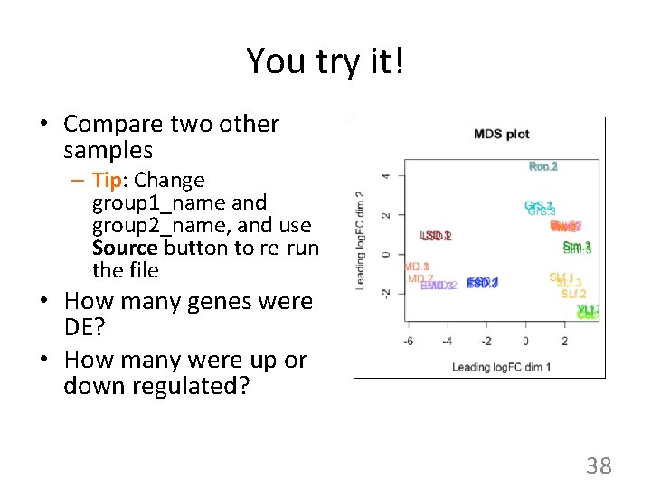
You try it! • Compare two other samples – Tip: Change group 1_name and group 2_name, and use Source button to re-run the file • How many genes were DE? • How many were up or down regulated? 38

Introduction to RNA-Seq • Describe assay & data produced • Describe differential expression analysis process • Describe confirmation/validation process – Check gene expression graphs in Genome Browser 39

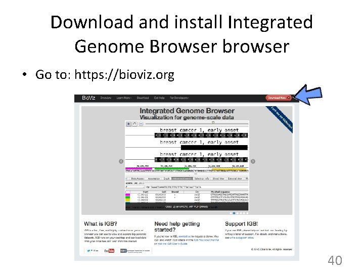
Download and install Integrated Genome Browser browser • Go to: https: //bioviz. org 40

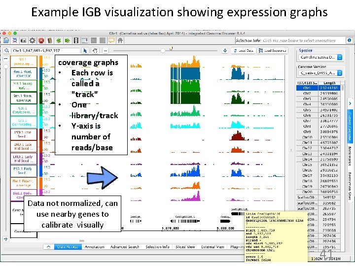
Example IGB visualization showing expression graphs coverage graphs • Each row is called a "track" • One library/track • Y-axis is number of reads/base Data not normalized, can use nearby genes to calibrate visually 41

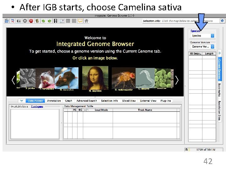
• After IGB starts, choose Camelina sativa 42

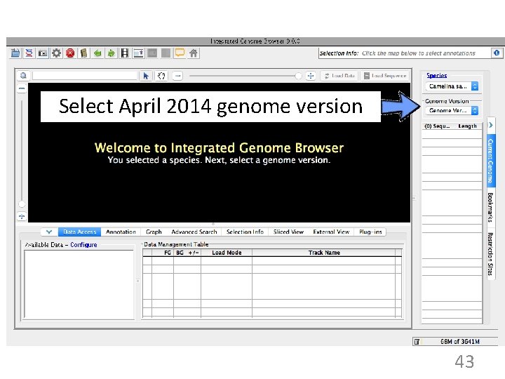
Select April 2014 genome version 43

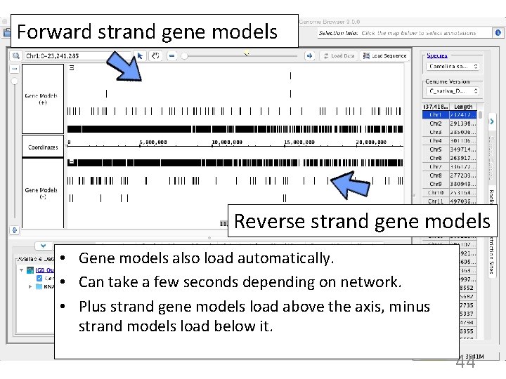
Forward strand gene models Reverse strand gene models • Gene models also load automatically. • Can take a few seconds depending on network. • Plus strand gene models load above the axis, minus strand models load below it. 44

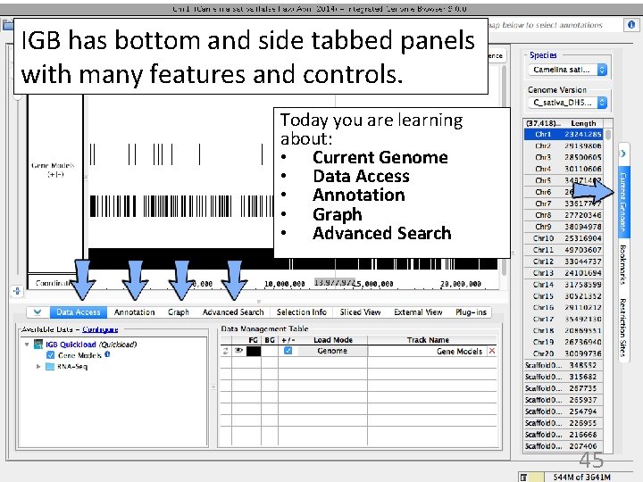
IGB has bottom and side tabbed panels with many features and controls. Today you are learning about: • Current Genome • Data Access • Annotation • Graph • Advanced Search 45

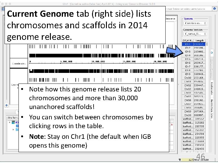
Current Genome tab (right side) lists chromosomes and scaffolds in 2014 genome release. • Note how this genome release lists 20 chromosomes and more than 30, 000 unanchored scaffolds! • You can switch between chromosomes by clicking rows in the table. • Note: Stay on Chr 1 (the default when IGB opens this genome) 46

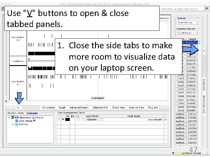
Use "V" buttons to open & close tabbed panels. 1. Close the side tabs to make more room to visualize data on your laptop screen. 47

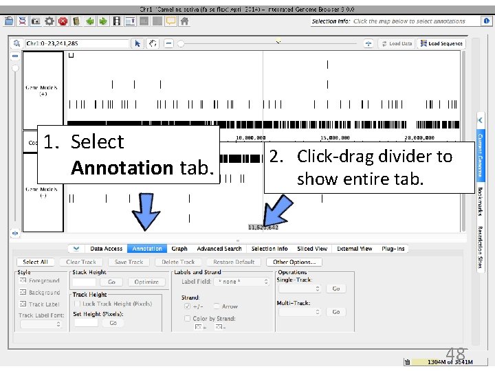
1. Select Annotation tab. 2. Click-drag divider to show entire tab. 48

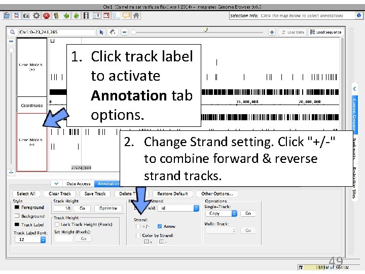
1. Click track label to activate Annotation tab options. 2. Change Strand setting. Click "+/-" to combine forward & reverse strand tracks. 49

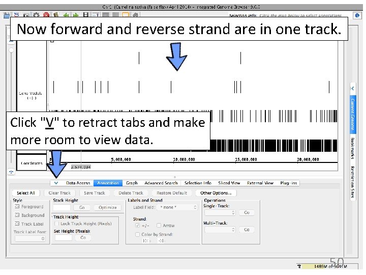
Now forward and reverse strand are in one track. Click "V" to retract tabs and make more room to view data. 50

IGB has many ways to move & zoom • Animated zooming – click to position zoom stripe, sets zoom focus – horizontal zoom & vertical stretch • Moving from side to side (panning) – arrows in toolbar – hand icon - the move tool • Jump-zooming – Click-drag coordinate axis with arrow tool – Double-click to zoom in on a feature – Search by name 51

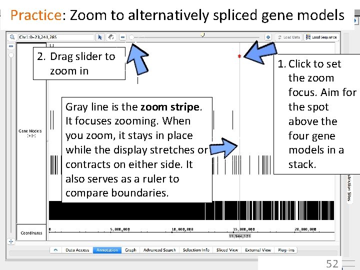
Practice: Zoom to alternatively spliced gene models 2. Drag slider to zoom in Gray line is the zoom stripe. It focuses zooming. When you zoom, it stays in place while the display stretches or contracts on either side. It also serves as a ruler to compare boundaries. * 1. Click to set the zoom focus. Aim for the spot above the four gene models in a stack. 52

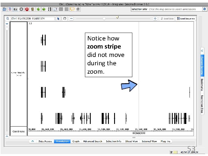
Notice how zoom stripe did not move during the zoom. 53

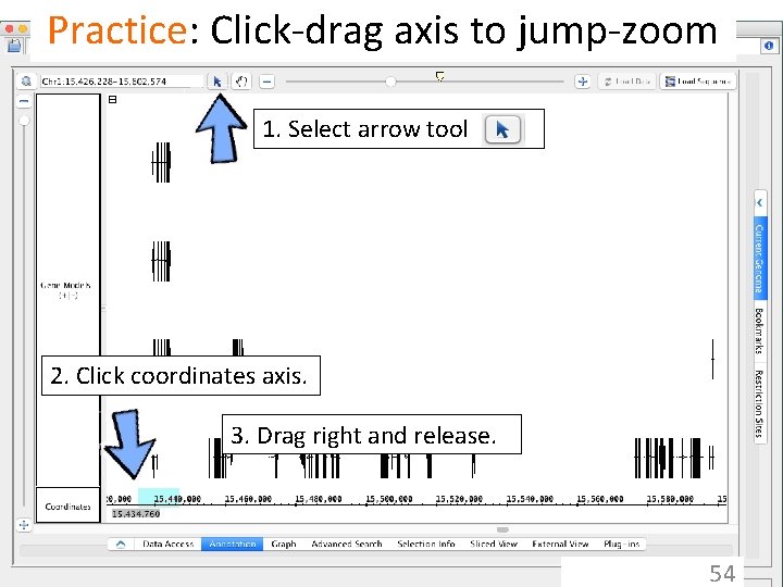
Practice: Click-drag axis to jump-zoom 1. Select arrow tool 2. Click coordinates axis. 3. Drag right and release. 54

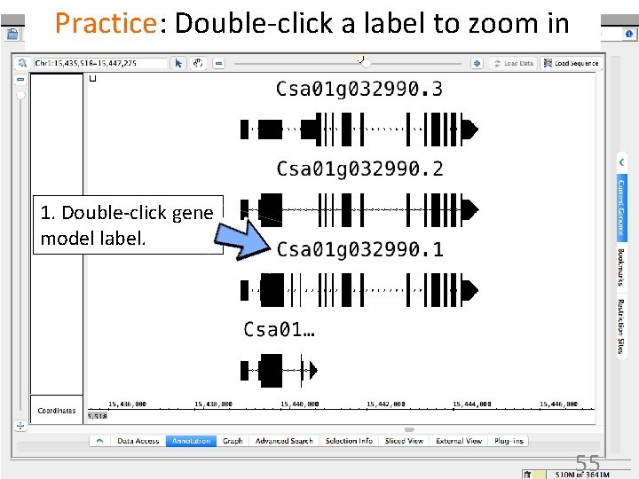
Practice: Double-click a label to zoom in 1. Double-click gene model label. 55

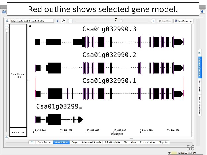
Red outline shows selected gene model. 56

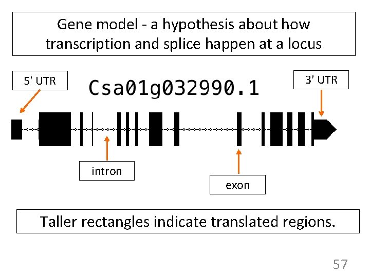
Gene model - a hypothesis about how transcription and splice happen at a locus 3' UTR 5' UTR intron exon Taller rectangles indicate translated regions. 57

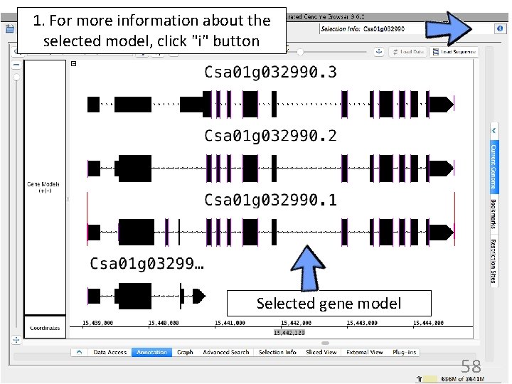
1. For more information about the selected model, click "i" button Selected gene model 58

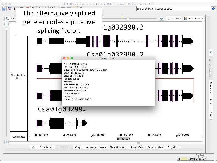
This alternatively spliced gene encodes a putative splicing factor. 59

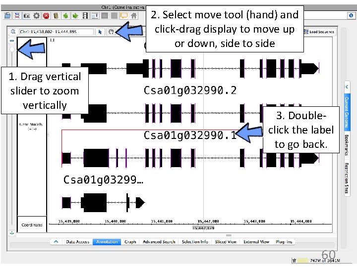
2. Select move tool (hand) and click-drag display to move up or down, side to side 1. Drag vertical slider to zoom vertically 3. Doubleclick the label to go back. 60

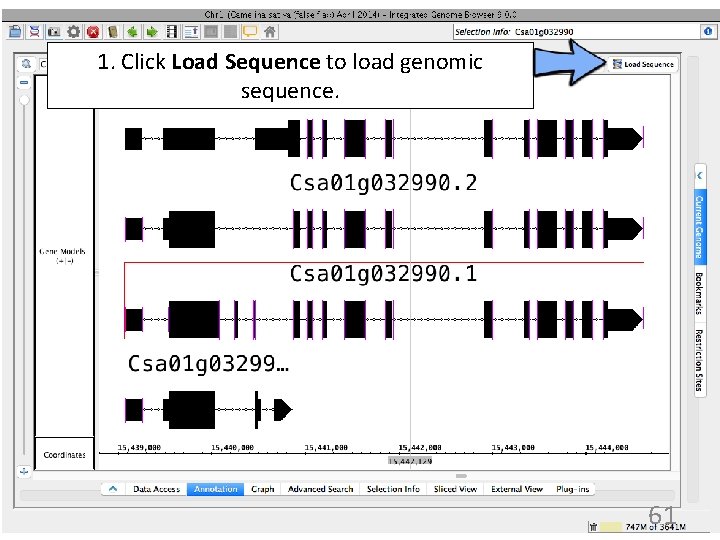
1. Click Load Sequence to load genomic sequence. 61

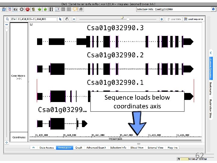
Sequence loads below coordinates axis 62

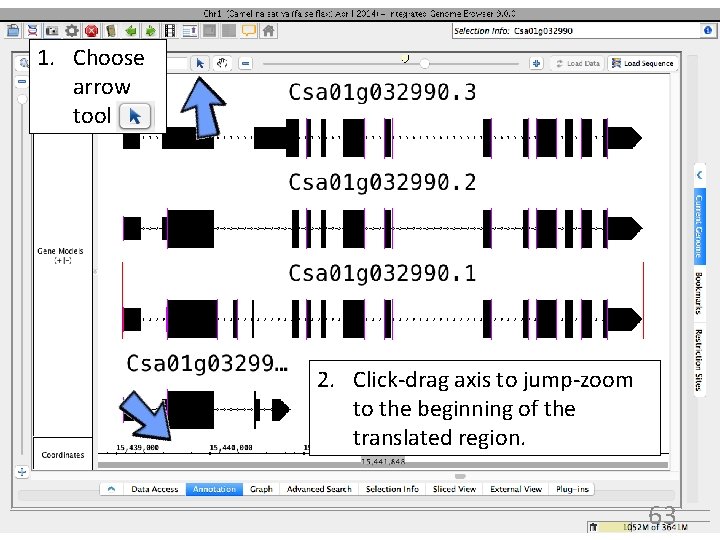
1. Choose arrow tool 2. Click-drag axis to jump-zoom to the beginning of the translated region. 63

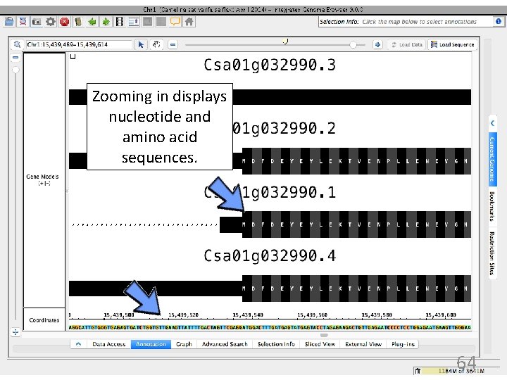
Zooming in displays nucleotide and amino acid sequences. 64

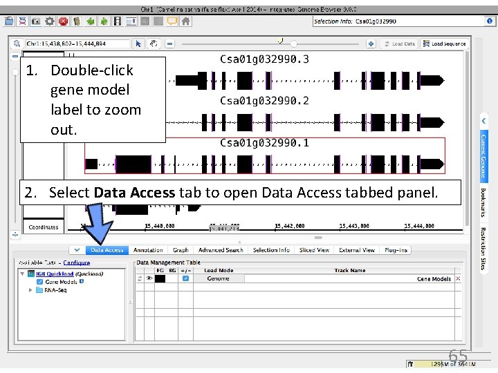
1. Double-click gene model label to zoom out. 2. Select Data Access tab to open Data Access tabbed panel. 65

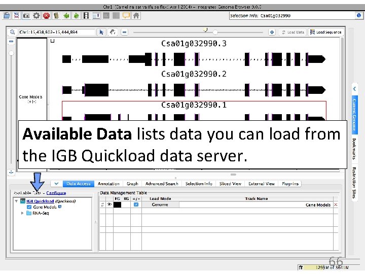
Available Data lists data you can load from the IGB Quickload data server. 66

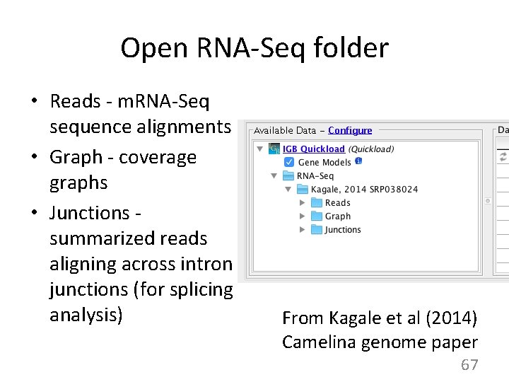
Open RNA-Seq folder • Reads - m. RNA-Seq sequence alignments • Graph - coverage graphs • Junctions summarized reads aligning across intron junctions (for splicing analysis) From Kagale et al (2014) Camelina genome paper 67

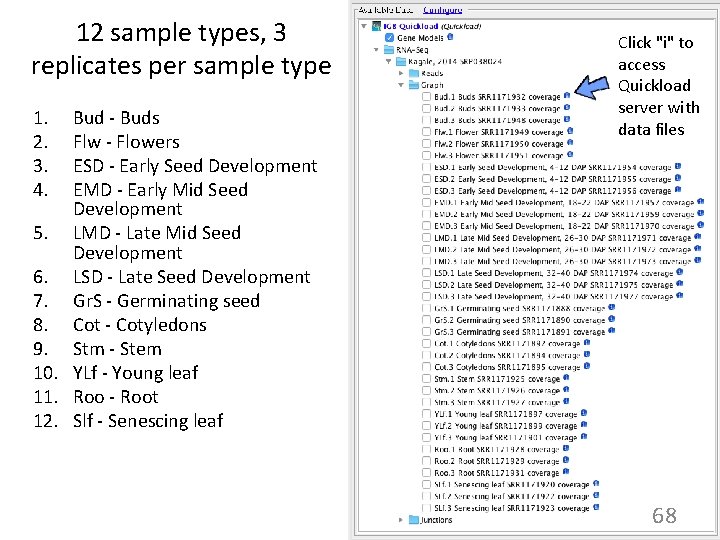
12 sample types, 3 replicates per sample type 1. 2. 3. 4. Bud - Buds Flw - Flowers ESD - Early Seed Development EMD - Early Mid Seed Development 5. LMD - Late Mid Seed Development 6. LSD - Late Seed Development 7. Gr. S - Germinating seed 8. Cot - Cotyledons 9. Stm - Stem 10. YLf - Young leaf 11. Roo - Root 12. Slf - Senescing leaf Click "i" to access Quickload server with data files 68

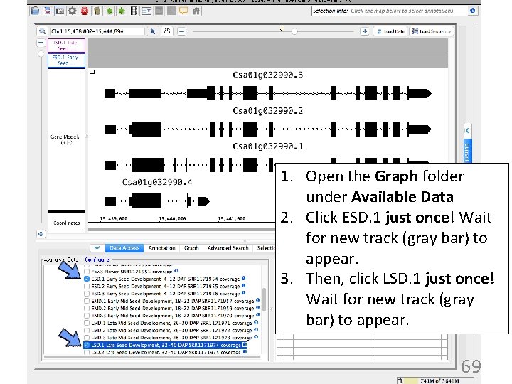
1. Open the Graph folder under Available Data 2. Click ESD. 1 just once! Wait for new track (gray bar) to appear. 3. Then, click LSD. 1 just once! Wait for new track (gray bar) to appear. 69

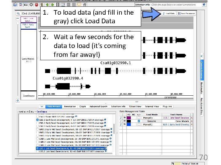
1. To load data (and fill in the gray) click Load Data 2. Wait a few seconds for the data to load (it's coming from far away!) 70

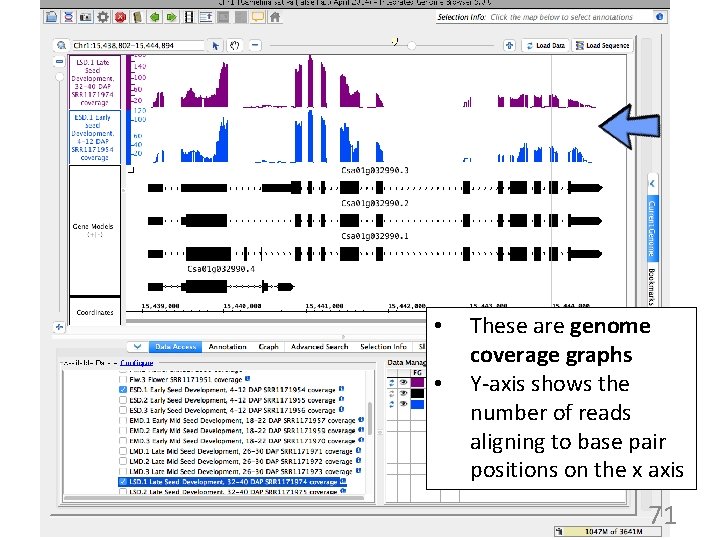
• • These are genome coverage graphs Y-axis shows the number of reads aligning to base pair positions on the x axis 71

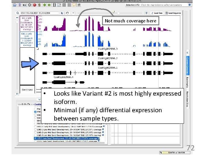
Not much coverage here • • Looks like Variant #2 is most highly expressed isoform. Minimal (if any) differential expression between sample types. 72

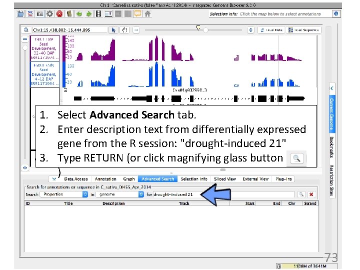
1. Select Advanced Search tab. 2. Enter description text from differentially expressed gene from the R session: "drought-induced 21" 3. Type RETURN (or click magnifying glass button ) 73

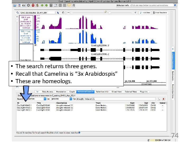
• The search returns three genes. • Recall that Camelina is “ 3 x Arabidospis” • These are homeologs. 74

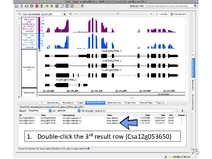
1. Double-click the 3 rd result row (Csa 12 g 053650) 75

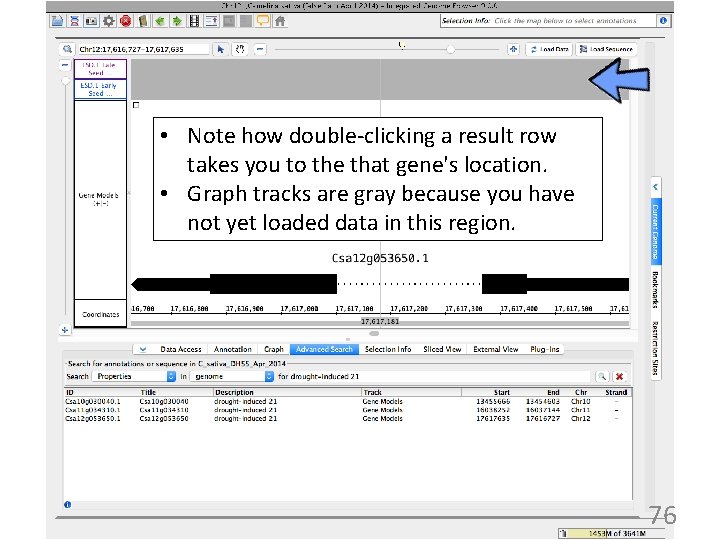
• Note how double-clicking a result row takes you to the that gene's location. • Graph tracks are gray because you have not yet loaded data in this region. 76

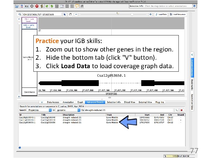
Practice your IGB skills: 1. Zoom out to show other genes in the region. 2. Hide the bottom tab (click "V" button). 3. Click Load Data to load coverage graph data. 77

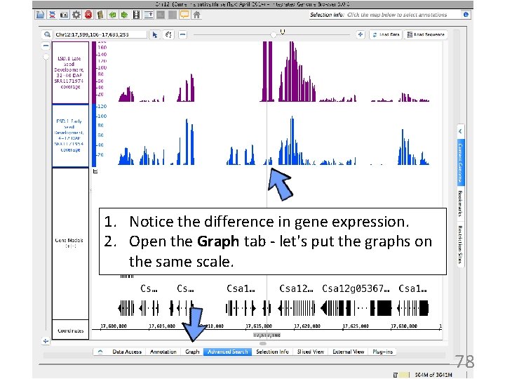
1. Notice the difference in gene expression. 2. Open the Graph tab - let's put the graphs on the same scale. 78

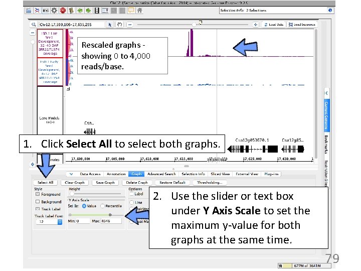
Rescaled graphs showing 0 to 4, 000 reads/base. 1. Click Select All to select both graphs. 2. Use the slider or text box under Y Axis Scale to set the maximum y-value for both graphs at the same time. 79

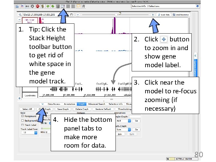
1. Tip: Click the Stack Height toolbar button to get rid of white space in the gene model track. 4. Hide the bottom panel tabs to make more room for data. 2. Click button to zoom in and show gene model label. 3. Click near the model to re-focus zooming (if necessary) 80

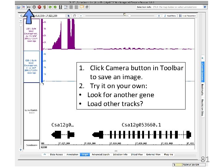
1. Click Camera button in Toolbar to save an image. 2. Try it on your own: • Look for another gene • Load other tracks? 81

Key idea: Visualize to validate & communicate & explore • Sanity-check your results – Did labels get switched? – Does the calculated fold-change make sense? • Create images to illustrate your findings • Explore – might discover something biologically meaningful – Zoom up and down, look at the data in different scales 82