Introduction to Regression Model Xueying Li MS Senior

Introduction to Regression Model Xueying Li, MS Senior Biostatistician Biostatistical Consulting Core (BCC) Stony Brook Cancer Center June 19, 2019 1

Outline v Linear regression model - Simple linear regression - Multiple linear regression v. Logistic regression model ©copyright reserved 2

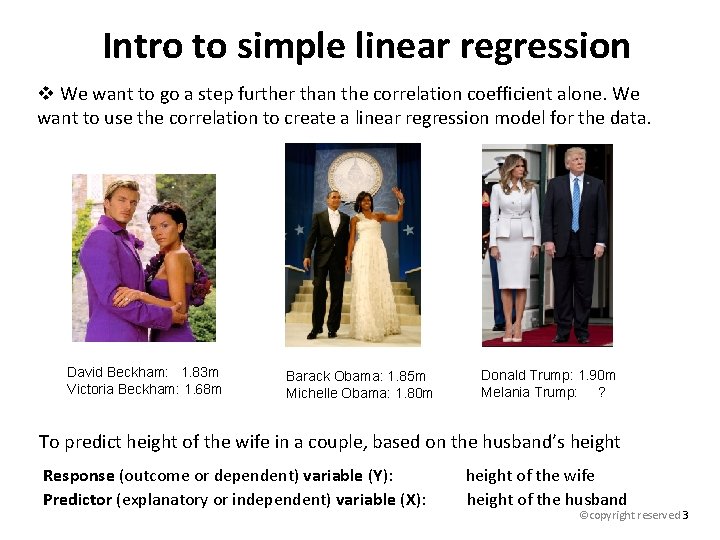
Intro to simple linear regression v We want to go a step further than the correlation coefficient alone. We want to use the correlation to create a linear regression model for the data. David Beckham: 1. 83 m Victoria Beckham: 1. 68 m Barack Obama: 1. 85 m Michelle Obama: 1. 80 m Donald Trump: 1. 90 m Melania Trump: ? To predict height of the wife in a couple, based on the husband’s height Response (outcome or dependent) variable (Y): height of the wife Predictor (explanatory or independent) variable (X): height of the husband ©copyright reserved 3

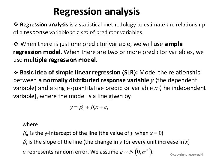
Regression analysis v Regression analysis is a statistical methodology to estimate the relationship of a response variable to a set of predictor variables. v When there is just one predictor variable, we will use simple regression model. When there are two or more predictor variables, we use multiple regression model. v Basic idea of simple linear regression (SLR): Model the relationship between a normally distributed response variable y (the dependent variable) and a single quantitative predictor variable x (the independent variable), where the model is a line given by ©copyright reserved 4

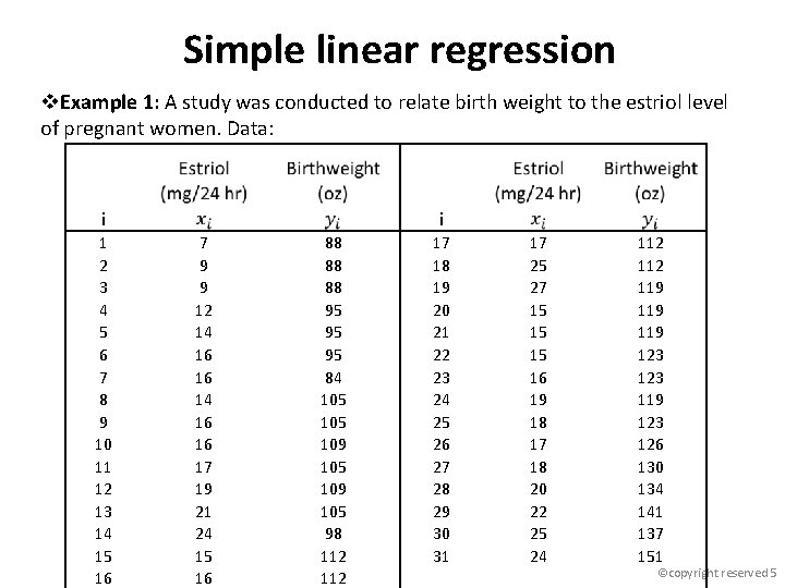
Simple linear regression v. Example 1: A study was conducted to relate birth weight to the estriol level of pregnant women. Data: i 1 2 3 4 5 6 7 8 9 10 11 12 13 14 15 16 i 7 9 9 12 14 16 16 17 19 21 24 15 16 88 88 88 95 95 95 84 105 109 105 98 112 17 18 19 20 21 22 23 24 25 26 27 28 29 30 31 17 25 27 15 15 15 16 19 18 17 18 20 22 25 24 112 119 119 123 126 130 134 141 137 151 ©copyright reserved 5

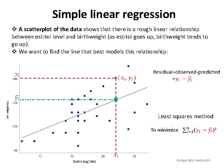
Simple linear regression v A scatterplot of the data shows that there is a rough linear relationship between estriol level and birthweight (as estriol goes up, birthweight tends to go up). v We want to find the line that best models this relationship: We want the equation of this line (that is, we want to estimate β 0 and β 1). Least squares method To minimize ©copyright reserved 6

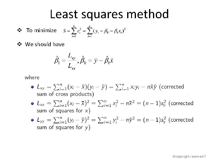
Least squares method v To minimize v We should have ©copyright reserved 7

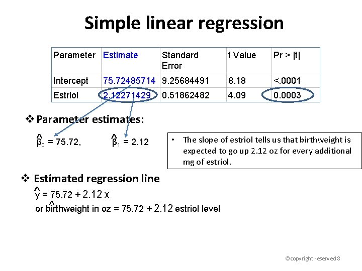
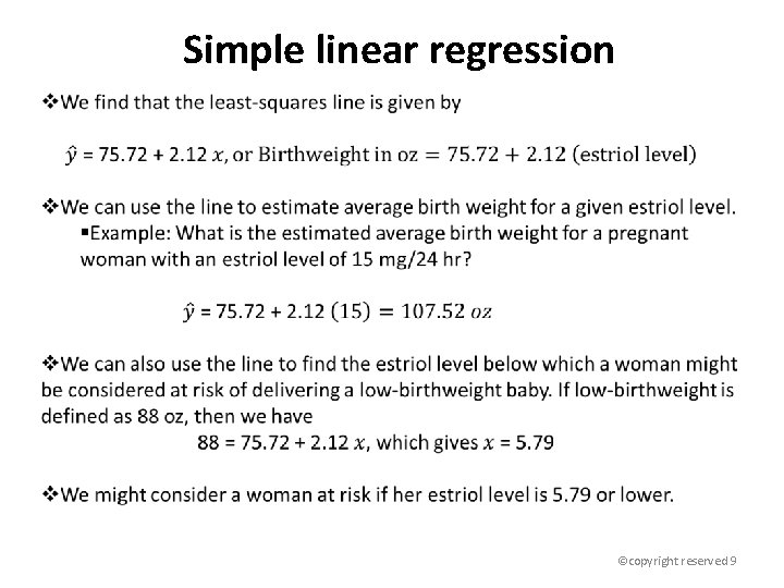
Simple linear regression Parameter Estimate Standard Error t Value Pr > |t| Intercept 75. 72485714 9. 25684491 8. 18 <. 0001 Estriol 2. 12271429 4. 09 0. 0003 0. 51862482 v. Parameter estimates: β 0 = 75. 72, β 1 = 2. 12 • The slope of estriol tells us that birthweight is expected to go up 2. 12 oz for every additional mg of estriol. v Estimated regression line y = 75. 72 + 2. 12 x or birthweight in oz = 75. 72 + 2. 12 estriol level ©copyright reserved 8

Simple linear regression ©copyright reserved 9

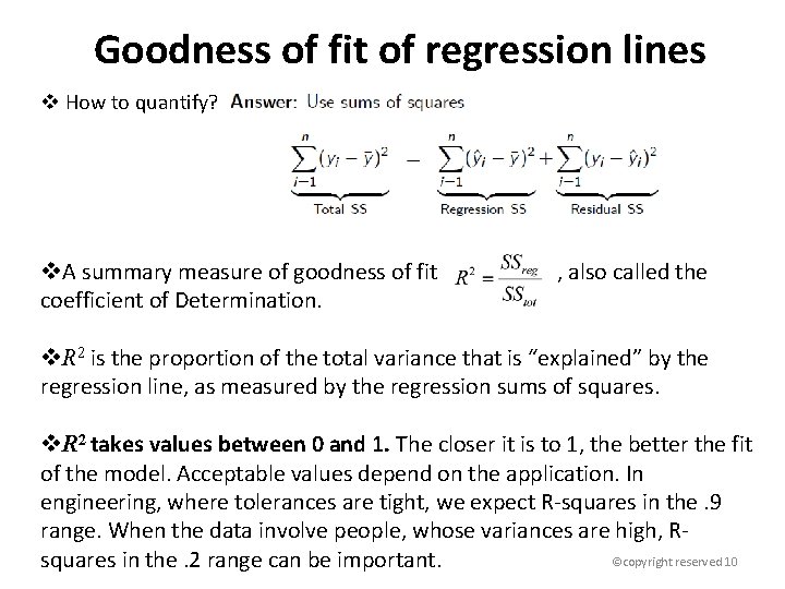
Goodness of fit of regression lines v How to quantify? v. A summary measure of goodness of fit , also called the coefficient of Determination. v. R 2 is the proportion of the total variance that is “explained” by the regression line, as measured by the regression sums of squares. v. R 2 takes values between 0 and 1. The closer it is to 1, the better the fit of the model. Acceptable values depend on the application. In engineering, where tolerances are tight, we expect R-squares in the. 9 range. When the data involve people, whose variances are high, R©copyright reserved 10 squares in the. 2 range can be important.

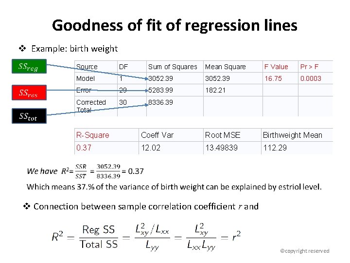
Goodness of fit of regression lines v Example: birth weight Source DF Sum of Squares Mean Square F Value Pr > F Model 1 3052. 39 16. 75 0. 0003 Error 29 5283. 99 182. 21 Corrected Total 30 8336. 39 R-Square Coeff Var Root MSE Birthweight Mean 0. 37 12. 02 13. 49839 112. 29 v Connection between sample correlation coefficient r and ©copyright reserved

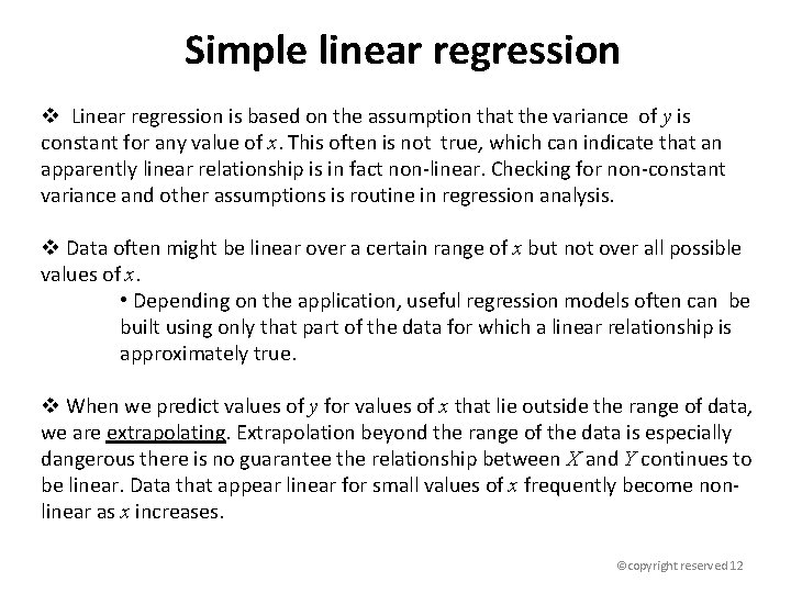
Simple linear regression v Linear regression is based on the assumption that the variance of y is constant for any value of x. This often is not true, which can indicate that an apparently linear relationship is in fact non-linear. Checking for non-constant variance and other assumptions is routine in regression analysis. v Data often might be linear over a certain range of x but not over all possible values of x. • Depending on the application, useful regression models often can be built using only that part of the data for which a linear relationship is approximately true. v When we predict values of y for values of x that lie outside the range of data, we are extrapolating. Extrapolation beyond the range of the data is especially dangerous there is no guarantee the relationship between X and Y continues to be linear. Data that appear linear for small values of x frequently become nonlinear as x increases. ©copyright reserved 12

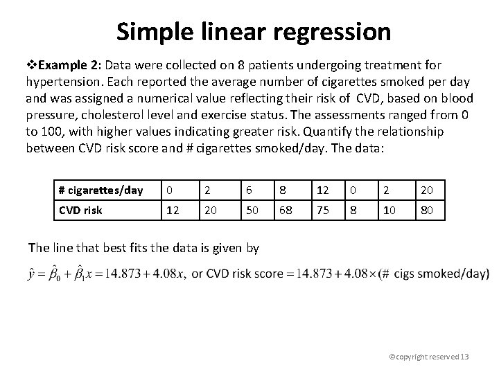
Simple linear regression v. Example 2: Data were collected on 8 patients undergoing treatment for hypertension. Each reported the average number of cigarettes smoked per day and was assigned a numerical value reflecting their risk of CVD, based on blood pressure, cholesterol level and exercise status. The assessments ranged from 0 to 100, with higher values indicating greater risk. Quantify the relationship between CVD risk score and # cigarettes smoked/day. The data: # cigarettes/day 0 2 6 8 12 0 2 20 CVD risk 12 20 50 68 75 8 10 80 The line that best fits the data is given by ©copyright reserved 13

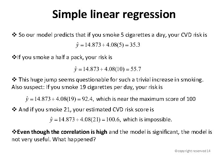
Simple linear regression v So our model predicts that if you smoke 5 cigarettes a day, your CVD risk is v. If you smoke a half a pack, your risk is v This huge jump seems questionable for such a trivial increase in smoking. Also suspect: If you smoke 19 cigarettes per day, your risk is v And if you smoke 21, your estimated CVD risk score is v. Even though the correlation is high and the model is significant, the model is not very useful. What happened? ©copyright reserved 14

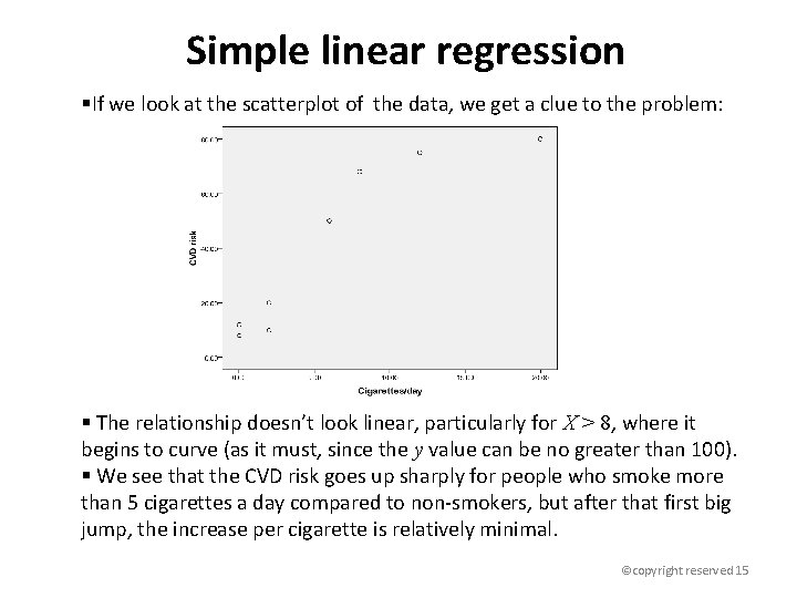
Simple linear regression §If we look at the scatterplot of the data, we get a clue to the problem: § The relationship doesn’t look linear, particularly for X > 8, where it begins to curve (as it must, since the y value can be no greater than 100). § We see that the CVD risk goes up sharply for people who smoke more than 5 cigarettes a day compared to non-smokers, but after that first big jump, the increase per cigarette is relatively minimal. ©copyright reserved 15

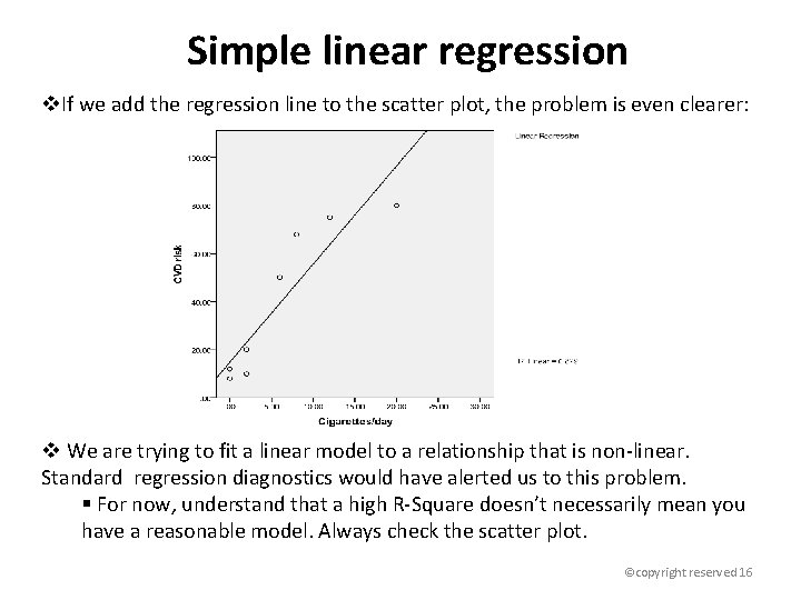
Simple linear regression v. If we add the regression line to the scatter plot, the problem is even clearer: v We are trying to fit a linear model to a relationship that is non-linear. Standard regression diagnostics would have alerted us to this problem. § For now, understand that a high R-Square doesn’t necessarily mean you have a reasonable model. Always check the scatter plot. ©copyright reserved 16

Multiple linear regression ©copyright reserved 17

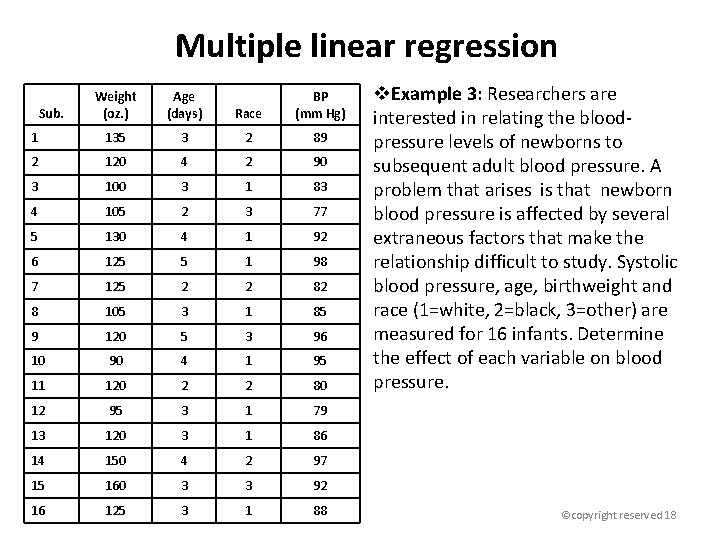
Multiple linear regression Weight (oz. ) Age (days) Race BP (mm Hg) 1 135 3 2 89 2 120 4 2 90 3 100 3 1 83 4 105 2 3 77 5 130 4 1 92 6 125 5 1 98 7 125 2 2 82 8 105 3 1 85 9 120 5 3 96 10 90 4 1 95 11 120 2 2 80 12 95 3 1 79 13 120 3 1 86 14 150 4 2 97 15 160 3 3 92 16 125 3 1 88 Sub. v. Example 3: Researchers are interested in relating the bloodpressure levels of newborns to subsequent adult blood pressure. A problem that arises is that newborn blood pressure is affected by several extraneous factors that make the relationship difficult to study. Systolic blood pressure, age, birthweight and race (1=white, 2=black, 3=other) are measured for 16 infants. Determine the effect of each variable on blood pressure. ©copyright reserved 18

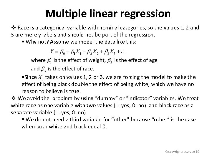
Multiple linear regression v Race is a categorical variable with nominal categories, so the values 1, 2 and 3 are merely labels and should not be part of the regression. § Why not? Assume we model the data like this: §Since X 3 takes on values 1, 2 or 3, we are forcing the model to make the effect of being black double the effect of being white, which we have no reason to believe is true. v We avoid the problem by using “dummy” or “indicator” variables. We treat white race as one variable with two values (1=yes, 0=no) and black race as a separate variable (1=yes, 0=no). § We do not need a third variable for “other” because “other” is the case when both white and black equal 0. ©copyright reserved 19

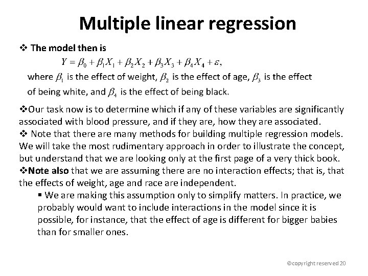
Multiple linear regression v The model then is v. Our task now is to determine which if any of these variables are significantly associated with blood pressure, and if they are, how they are associated. v Note that there are many methods for building multiple regression models. We will take the most rudimentary approach in order to illustrate the concept, but understand that we are looking only at the first page of a very thick book. v. Note also that we are assuming there are no interaction effects; that is, that the effects of weight, age and race are independent. § We are making this assumption only to simplify matters. In practice, we probably would want to include interactions in the model since it is possible, for instance, that the effect of age is different for bigger babies than for smaller ones. ©copyright reserved 20

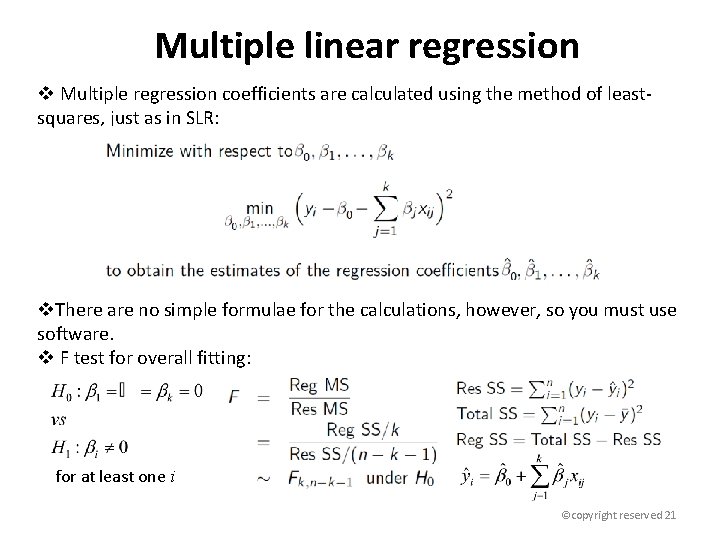
Multiple linear regression v Multiple regression coefficients are calculated using the method of leastsquares, just as in SLR: v. There are no simple formulae for the calculations, however, so you must use software. v F test for overall fitting: for at least one i ©copyright reserved 21

Test for specific variables v v ©copyright reserved 22

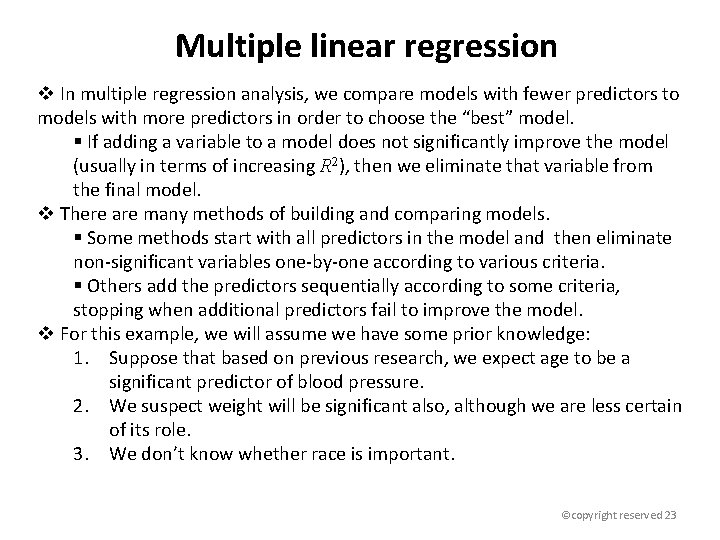
Multiple linear regression v In multiple regression analysis, we compare models with fewer predictors to models with more predictors in order to choose the “best” model. § If adding a variable to a model does not significantly improve the model (usually in terms of increasing R 2), then we eliminate that variable from the final model. v There are many methods of building and comparing models. § Some methods start with all predictors in the model and then eliminate non-significant variables one-by-one according to various criteria. § Others add the predictors sequentially according to some criteria, stopping when additional predictors fail to improve the model. v For this example, we will assume we have some prior knowledge: 1. Suppose that based on previous research, we expect age to be a significant predictor of blood pressure. 2. We suspect weight will be significant also, although we are less certain of its role. 3. We don’t know whether race is important. ©copyright reserved 23

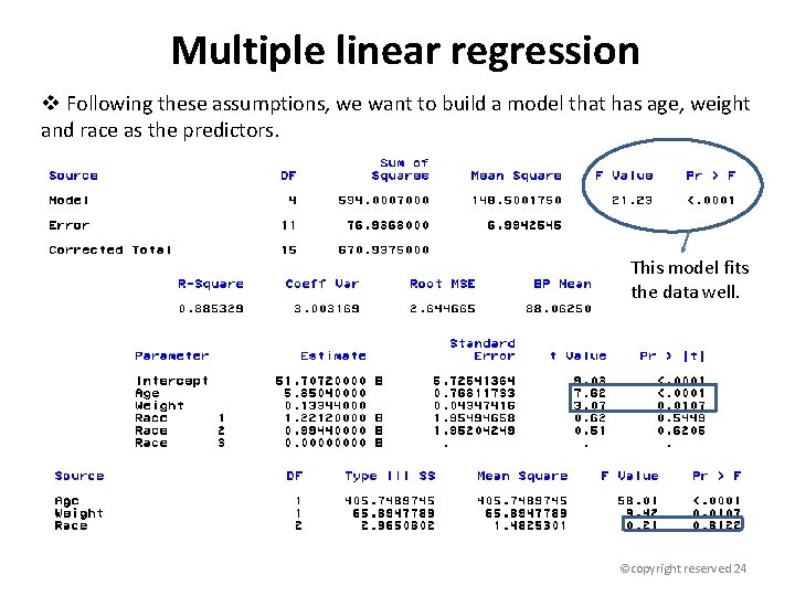
Multiple linear regression v Following these assumptions, we want to build a model that has age, weight and race as the predictors. This model fits the data well. ©copyright reserved 24

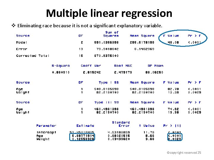
Multiple linear regression v Eliminating race because it is not a significant explanatory variable. ©copyright reserved 25

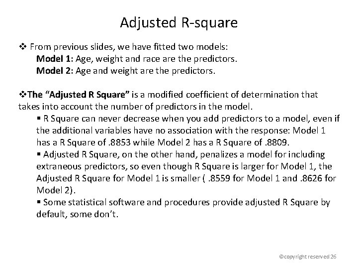
Adjusted R-square v From previous slides, we have fitted two models: Model 1: Age, weight and race are the predictors. Model 2: Age and weight are the predictors. v. The “Adjusted R Square” is a modified coefficient of determination that takes into account the number of predictors in the model. § R Square can never decrease when you add predictors to a model, even if the additional variables have no association with the response: Model 1 has a R Square of. 8853 while Model 2 has a R Square of. 8809. § Adjusted R Square, on the other hand, penalizes a model for including extraneous predictors, so even though R Square is larger for Model 1, the Adjusted R Square for Model 1 is smaller (. 8559 for Model 1 and. 8626 for Model 2). § Some statistical software and procedures provide adjusted R Square by default, some don’t. ©copyright reserved 26

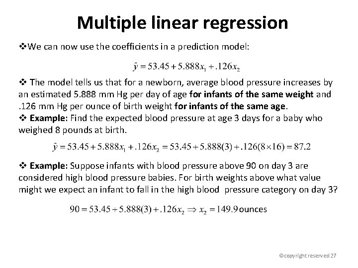
Multiple linear regression v. We can now use the coefficients in a prediction model: v The model tells us that for a newborn, average blood pressure increases by an estimated 5. 888 mm Hg per day of age for infants of the same weight and . 126 mm Hg per ounce of birth weight for infants of the same age. v Example: Find the expected blood pressure at age 3 days for a baby who weighed 8 pounds at birth. v Example: Suppose infants with blood pressure above 90 on day 3 are considered high blood pressure babies. For birth weights above what value might we expect an infant to fall in the high blood pressure category on day 3? ©copyright reserved 27

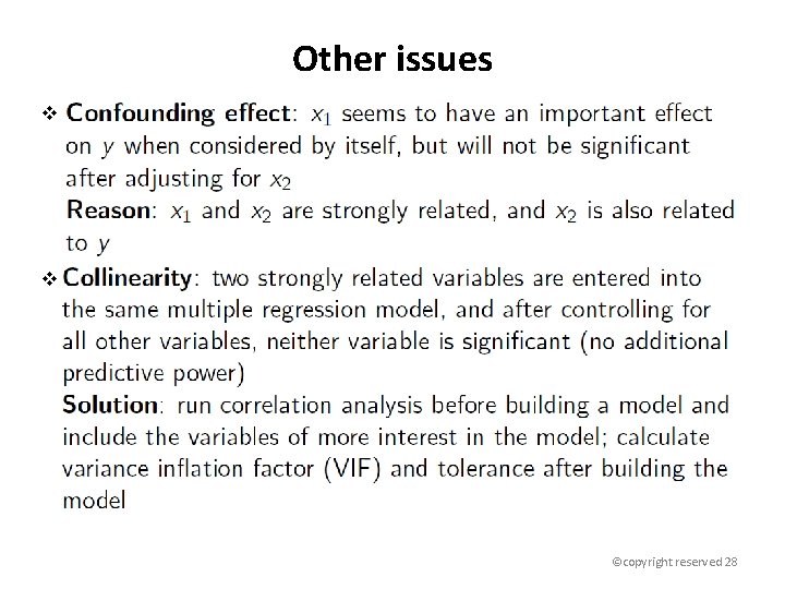
Other issues v v ©copyright reserved 28

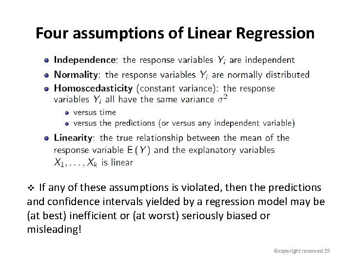
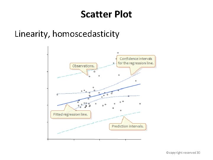
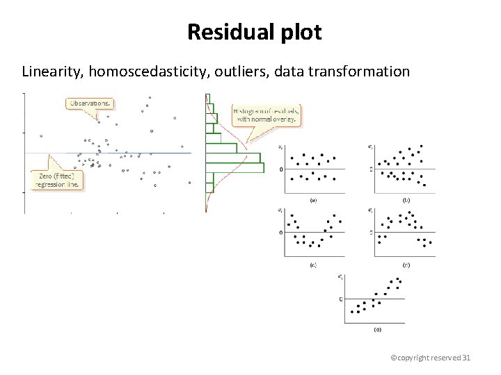
Four assumptions of Linear Regression v If any of these assumptions is violated, then the predictions and confidence intervals yielded by a regression model may be (at best) inefficient or (at worst) seriously biased or misleading! ©copyright reserved 29

Scatter Plot Linearity, homoscedasticity ©copyright reserved 30

Residual plot Linearity, homoscedasticity, outliers, data transformation ©copyright reserved 31

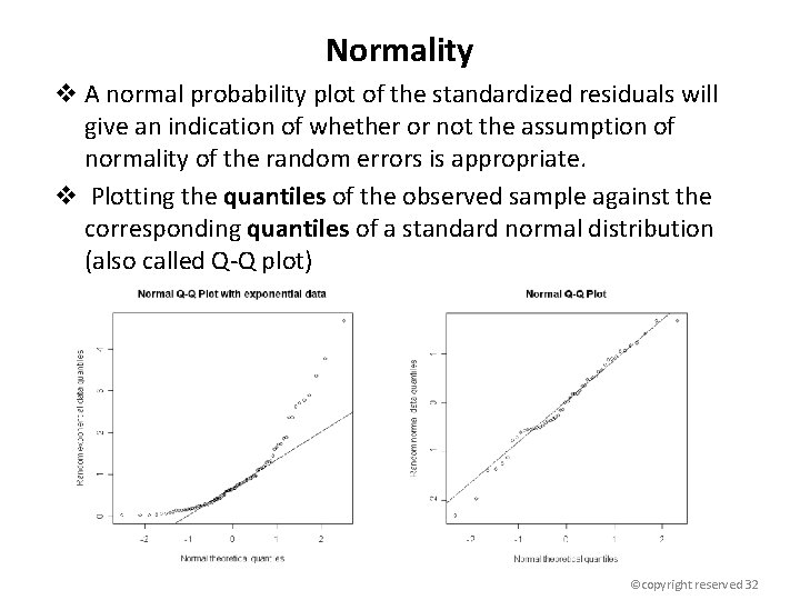
Normality v A normal probability plot of the standardized residuals will give an indication of whether or not the assumption of normality of the random errors is appropriate. v Plotting the quantiles of the observed sample against the corresponding quantiles of a standard normal distribution (also called Q-Q plot) ©copyright reserved 32

Outliers v When a possible outlier is detected, one should always try and find out v v v a reason If you have collected the data yourself, or have access to additional information about the data collection, you might be able to avoid the outlier (e. g. by correcting a misprint, or introducing an extra explanatory variable) When no explanation can be found, one has to decide whether to leave or omit the corresponding observation Report model results both with and without the outliers or to see how much they change Alternatively, it is sometimes possible to transform the data in such a way that outlying points are pulled closer towards the general trend in the transformed data Or consider nonparametric method Identification of outliers: if a standardized residual > 2 or <-2, then the corresponding observation may be regarded an outlier. ©copyright reserved 33

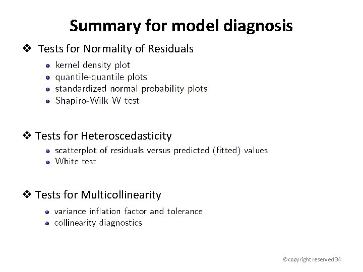
Summary for model diagnosis v Tests for Normality of Residuals v Tests for Heteroscedasticity v Tests for Multicollinearity ©copyright reserved 34

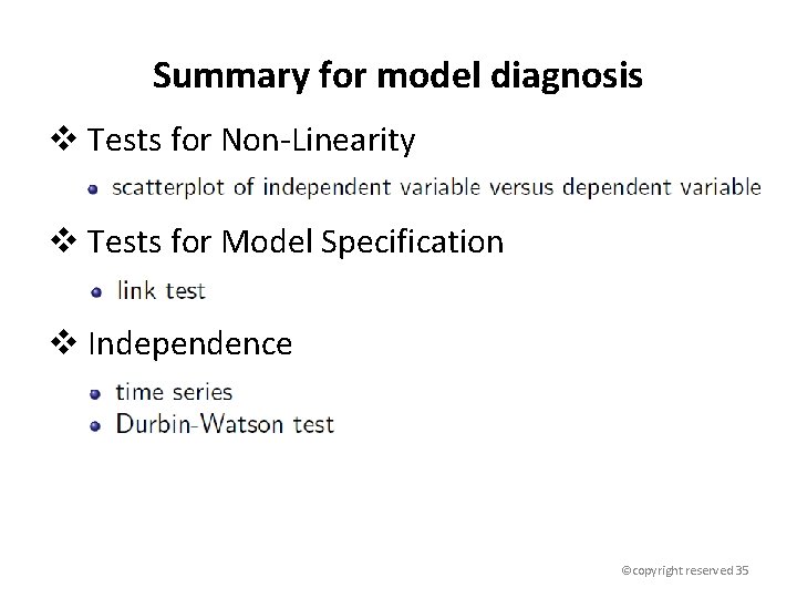
Summary for model diagnosis v Tests for Non-Linearity v Tests for Model Specification v Independence ©copyright reserved 35

LOGISTIC REGRESSION 36

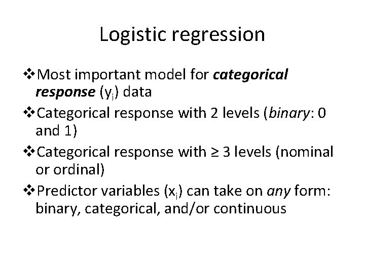
Logistic regression v. Most important model for categorical response (yi) data v. Categorical response with 2 levels (binary: 0 and 1) v. Categorical response with ≥ 3 levels (nominal or ordinal) v. Predictor variables (xi) can take on any form: binary, categorical, and/or continuous

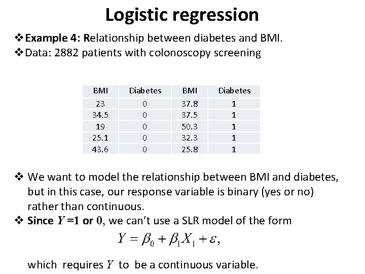
Logistic regression v. Example 4: Relationship between diabetes and BMI. v. Data: 2882 patients with colonoscopy screening BMI 23 34. 5 19 25. 1 43. 6 Diabetes 0 0 0 BMI 37. 8 37. 5 50. 3 32. 3 25. 8 Diabetes 1 1 1 v We want to model the relationship between BMI and diabetes, but in this case, our response variable is binary (yes or no) rather than continuous. v Since Y =1 or 0, we can’t use a SLR model of the form which requires Y to be a continuous variable.

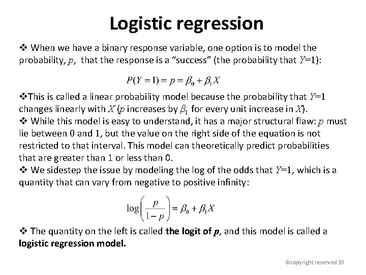
Logistic regression v When we have a binary response variable, one option is to model the probability, p, that the response is a “success” (the probability that Y=1): v. This is called a linear probability model because the probability that Y=1 changes linearly with X (p increases by β 1 for every unit increase in X). v While this model is easy to understand, it has a major structural flaw: p must lie between 0 and 1, but the value on the right side of the equation is not restricted to that interval. This model can theoretically predict probabilities that are greater than 1 or less than 0. v We sidestep the issue by modeling the log of the odds that Y=1, which is a quantity that can vary from negative to positive infinity: v The quantity on the left is called the logit of p, and this model is called a logistic regression model. ©copyright reserved 39

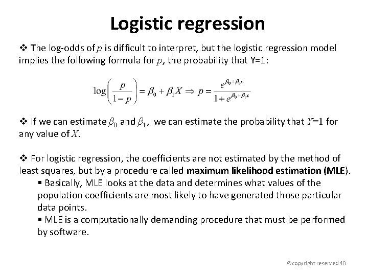
Logistic regression v The log-odds of p is difficult to interpret, but the logistic regression model implies the following formula for p, the probability that Y=1: v If we can estimate β 0 and β 1, we can estimate the probability that Y=1 for any value of X. v For logistic regression, the coefficients are not estimated by the method of least squares, but by a procedure called maximum likelihood estimation (MLE). § Basically, MLE looks at the data and determines what values of the population coefficients are most likely to have generated those particular data points. § MLE is a computationally demanding procedure that must be performed by software. ©copyright reserved 40

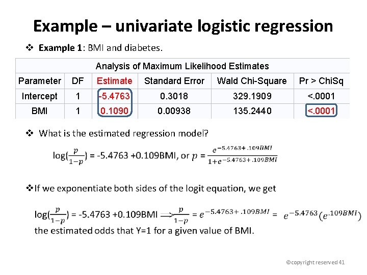
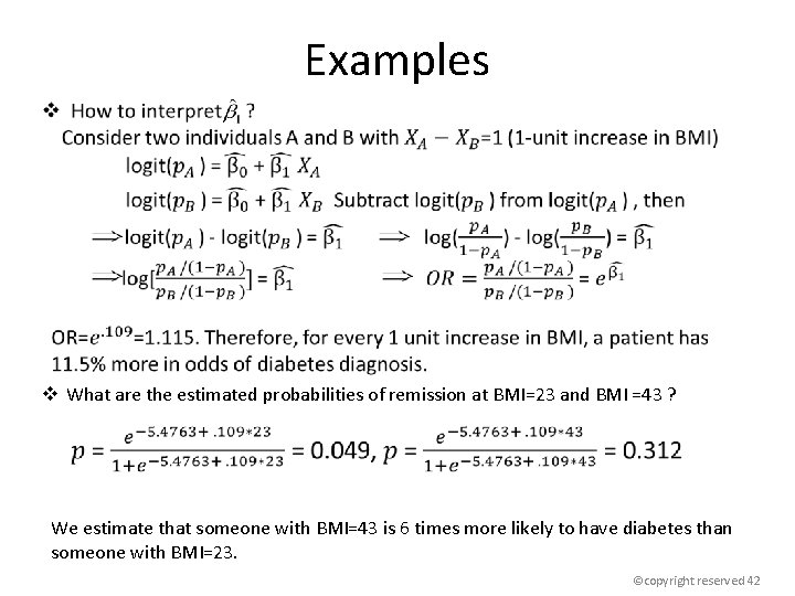
Example – univariate logistic regression v Example 1: BMI and diabetes. Analysis of Maximum Likelihood Estimates Parameter DF Estimate Standard Error Wald Chi-Square Pr > Chi. Sq Intercept 1 -5. 4763 0. 3018 329. 1909 <. 0001 BMI 1 0. 1090 0. 00938 135. 2440 <. 0001 v What is the estimated regression model? ©copyright reserved 41

Examples v What are the estimated probabilities of remission at BMI=23 and BMI =43 ? We estimate that someone with BMI=43 is 6 times more likely to have diabetes than someone with BMI=23. ©copyright reserved 42

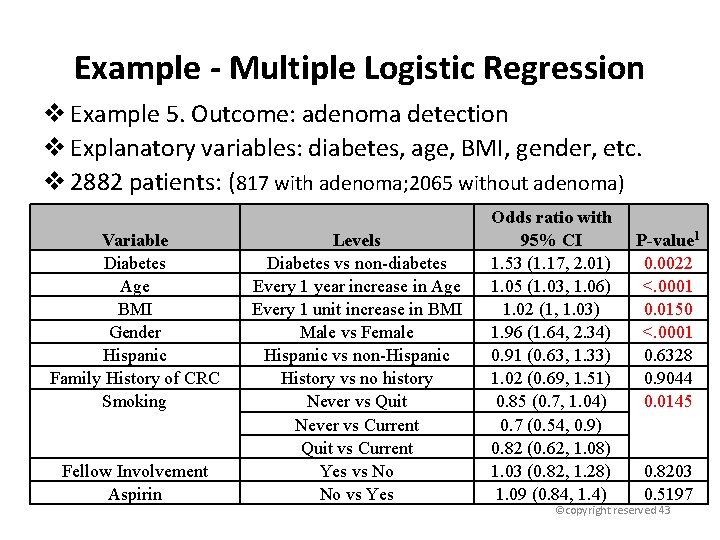
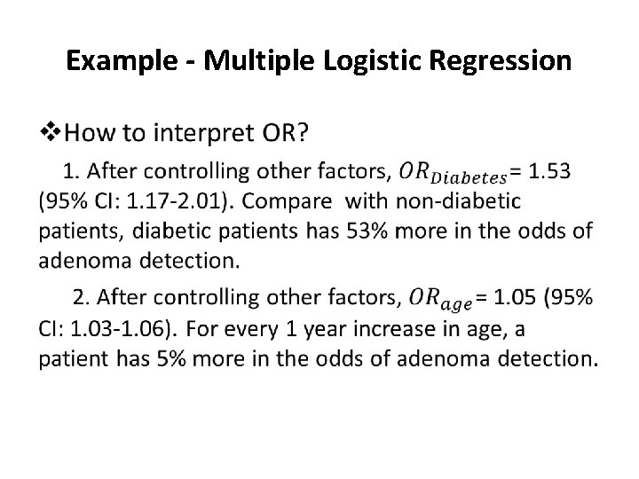
Example - Multiple Logistic Regression v Example 5. Outcome: adenoma detection v Explanatory variables: diabetes, age, BMI, gender, etc. v 2882 patients: (817 with adenoma; 2065 without adenoma) Variable Diabetes Age BMI Gender Hispanic Family History of CRC Smoking Fellow Involvement Aspirin Levels Diabetes vs non-diabetes Every 1 year increase in Age Every 1 unit increase in BMI Male vs Female Hispanic vs non-Hispanic History vs no history Never vs Quit Never vs Current Quit vs Current Yes vs No No vs Yes Odds ratio with 95% CI 1. 53 (1. 17, 2. 01) 1. 05 (1. 03, 1. 06) 1. 02 (1, 1. 03) 1. 96 (1. 64, 2. 34) 0. 91 (0. 63, 1. 33) 1. 02 (0. 69, 1. 51) 0. 85 (0. 7, 1. 04) 0. 7 (0. 54, 0. 9) 0. 82 (0. 62, 1. 08) 1. 03 (0. 82, 1. 28) 1. 09 (0. 84, 1. 4) P-value 1 0. 0022 <. 0001 0. 0150 <. 0001 0. 6328 0. 9044 0. 0145 0. 8203 0. 5197 ©copyright reserved 43

Example - Multiple Logistic Regression •

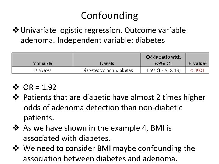
Confounding v Univariate logistic regression. Outcome variable: adenoma. Independent variable: diabetes Variable Diabetes Levels Diabetes vs non-diabetes Odds ratio with 95% CI 1. 92 (1. 49, 2. 48) P-value 1 <. 0001 v OR = 1. 92 v Patients that are diabetic have almost 2 times higher odds of adenoma detection than non-diabetic patients. v As we have shown in the example 4, BMI is associated with diabetes. v We need to consider BMI maybe confounding the association between diabetes and adenoma.

Confounding v When BMI is considered, these data suggest a weaker association between diabetes and adenoma. v If we did not control for BMI, then there would be a bias in the estimates of the diabetes-adenoma association. v Confounding variables must satisfy two conditions: - the exposure (diabetes) and confounding variables (BMI) are associated - the confounding variable itself is associated with the outcome (adenoma)

Summary v Logistic regression is used when the response variable, Y, is dichotomous. v Modeling the probability with a logistic function is equivalent to fitting a linear regression model in which the continuous response has been replaced by the logarithm of the odds of success for a dichotomous random variable. v Instead of assuming that the relationship between p and X is linear, we assume that the relationship between and X is linear. v Interpretation of coefficients depends on the type of the explanatory variables. v Conversion of estimated coefficients to estimated odds ratios v Hypothesis tests and confidence intervals for estimated regression coefficients No relationship→H 0 : ©copyright reserved 47