Introduction to Radial Basis Function Networks Contents l
Introduction to Radial Basis Function Networks
Contents l l l l l Overview The Models of Function Approximator The Radial Basis Function Networks RBFN’s for Function Approximation The Projection Matrix Learning the Kernels Bias-Variance Dilemma The Effective Number of Parameters Model Selection
RBF l l Linear models have been studied in statistics for about 200 years and theory is applicable to RBF networks which are just one particular type of linear model. However, the fashion for neural networks which started in the mid-80 has given rise to new names for concepts already familiar to statisticians
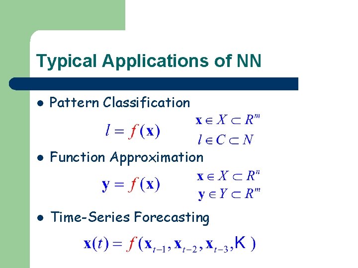
Typical Applications of NN l Pattern Classification l Function Approximation l Time-Series Forecasting
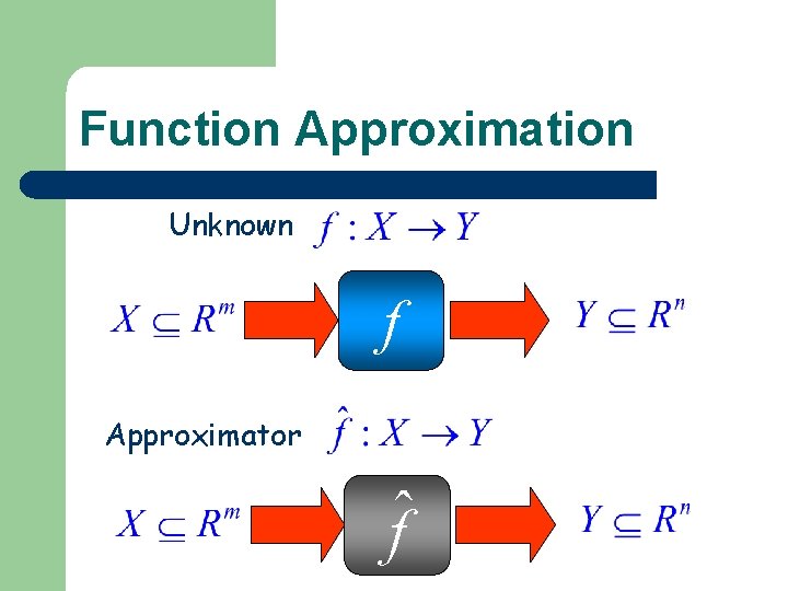
Function Approximation Unknown f Approximator ˆf
Introduction to Radial Basis Function Networks The Model of Function Approximator
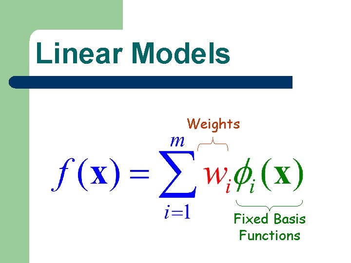
Linear Models Weights Fixed Basis Functions
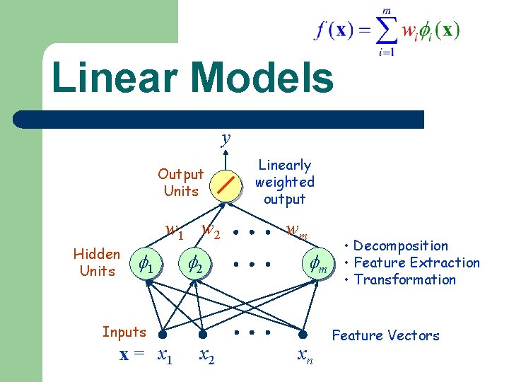
Linear Models y Output Units w 1 w 2 Hidden Units 1 2 Linearly weighted output wm m Inputs x = x 1 x 2 xn • Decomposition • Feature Extraction • Transformation Feature Vectors
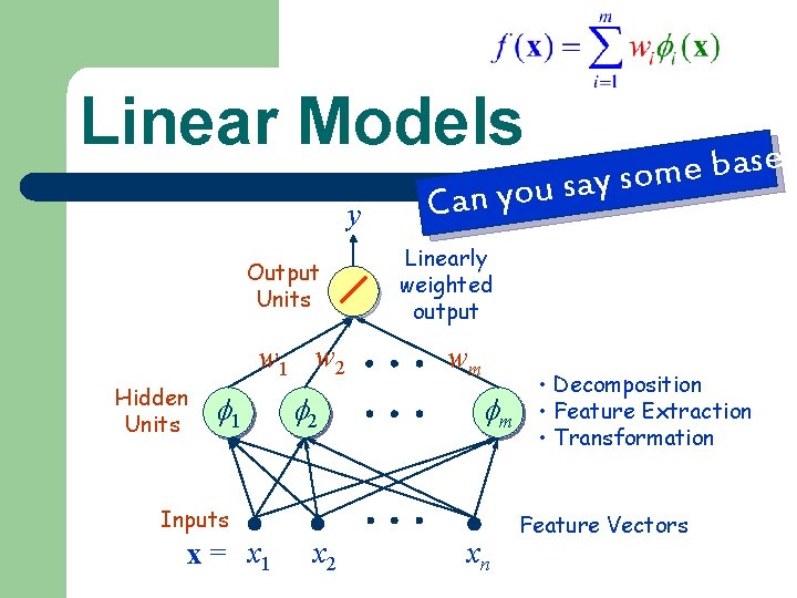
Linear Models y Output Units w 1 w 2 Hidden Units 1 2 Can you Linearly weighted output wm m Inputs x = x 1 x 2 s e s a b e say som xn • Decomposition • Feature Extraction • Transformation Feature Vectors
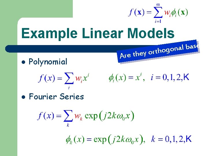
Example Linear Models l Polynomial l Fourier Series Are they ? s e s a b l a orthogon
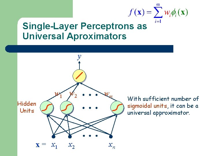
Single-Layer Perceptrons as Universal Aproximators y w 1 w 2 Hidden Units 1 x = x 1 2 x 2 wm m xn With sufficient number of sigmoidal units, it can be a universal approximator.
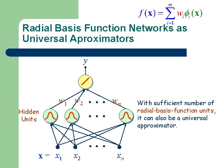
Radial Basis Function Networks as Universal Aproximators y w 1 w 2 Hidden Units 1 x = x 1 2 x 2 wm m xn With sufficient number of radial-basis-function units, it can also be a universal approximator.
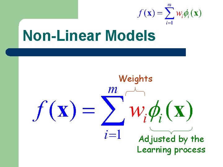
Non-Linear Models Weights Adjusted by the Learning process
Introduction to Radial Basis Function Networks The Radial Basis Function Networks
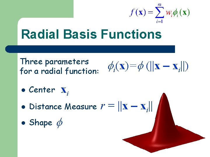
Radial Basis Functions Three parameters for a radial function: i(x)= (||x xi||) xi l Center l Distance Measure l Shape r = ||x xi||
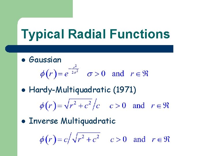
Typical Radial Functions l Gaussian l Hardy-Multiquadratic (1971) l Inverse Multiquadratic
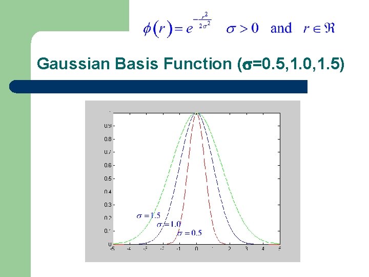
Gaussian Basis Function ( =0. 5, 1. 0, 1. 5)
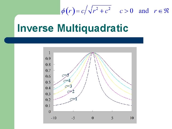
Inverse Multiquadratic c=5 c=4 c=3 c=2 c=1
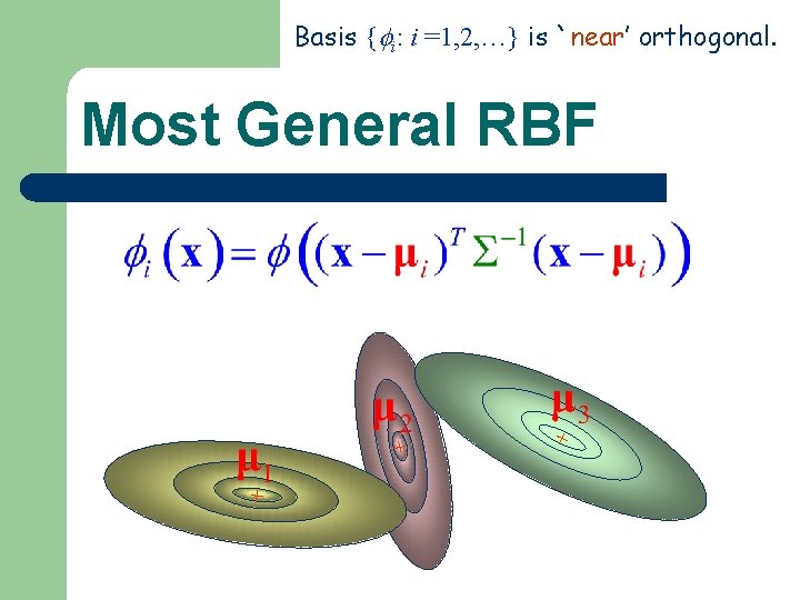
Basis { i: i =1, 2, …} is `near’ orthogonal. Most General RBF + + +
Properties of RBF’s l l On-Center, Off Surround Analogies with localized receptive fields found in several biological structures, e. g. , – – visual cortex; ganglion cells
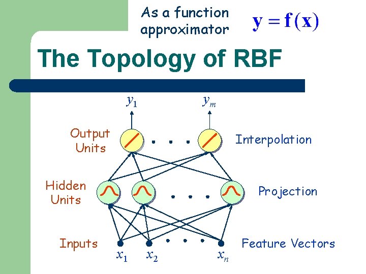
As a function approximator The Topology of RBF y 1 ym Output Units Interpolation Hidden Units Inputs Projection x 1 x 2 xn Feature Vectors
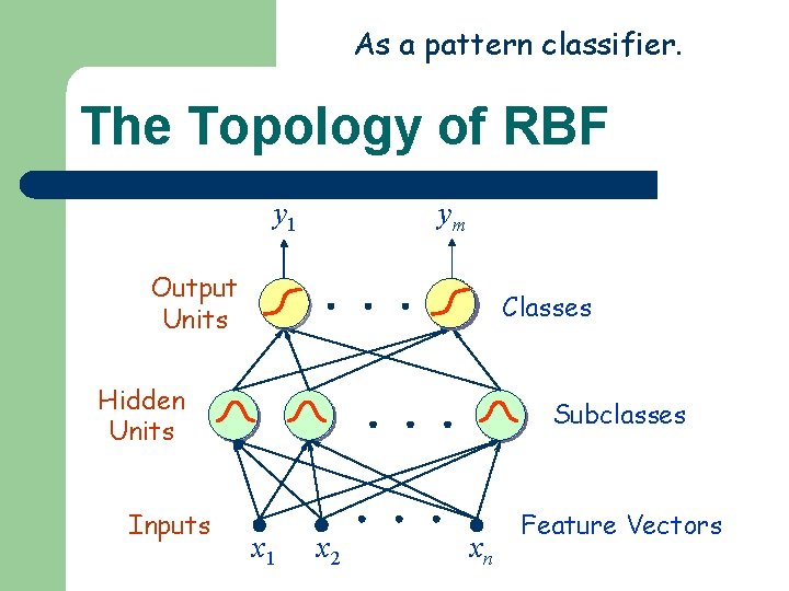
As a pattern classifier. The Topology of RBF y 1 ym Output Units Classes Hidden Units Inputs Subclasses x 1 x 2 xn Feature Vectors
Introduction to Radial Basis Function Networks RBFN’s for Function Approximation
Radial Basis Function Networks l l Radial basis function (RBF) networks are feedforward networks trained using a supervised training algorithm. The activation function is selected from a class of functions called basis functions. They usually train much faster than BP. They are less susceptible to problems with nonstationary inputs
Radial Basis Function Networks l l l Popularized by Broomhead and Lowe (1988), and Moody and Darken (1989), RBF networks have proven to be a useful neural network architecture. The major difference between RBF and BP is the behavior of the single hidden layer. Rather than using the sigmoidal or S-shaped activation function as in BP, the hidden units in RBF networks use a Gaussian or some other basis kernel function.
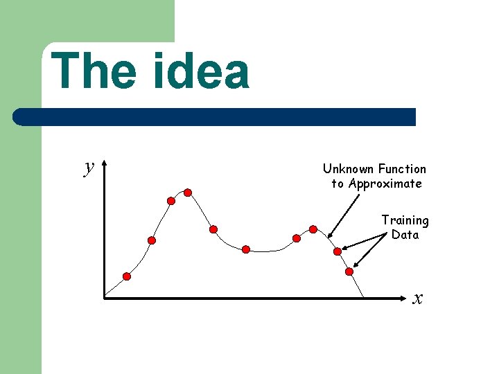
The idea y Unknown Function to Approximate Training Data x
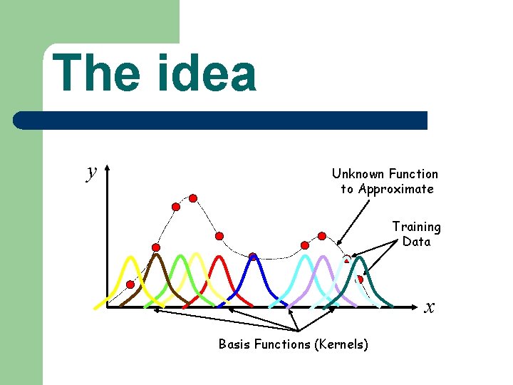
The idea y Unknown Function to Approximate Training Data x Basis Functions (Kernels)
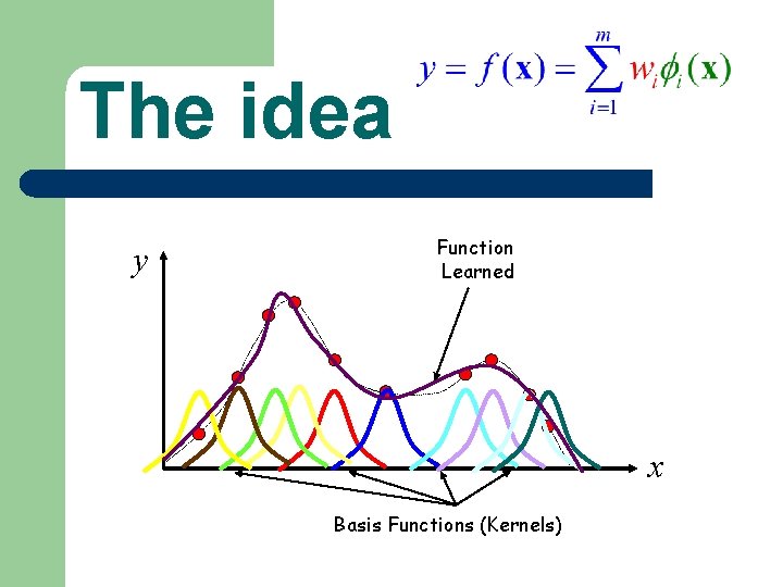
The idea y Function Learned x Basis Functions (Kernels)
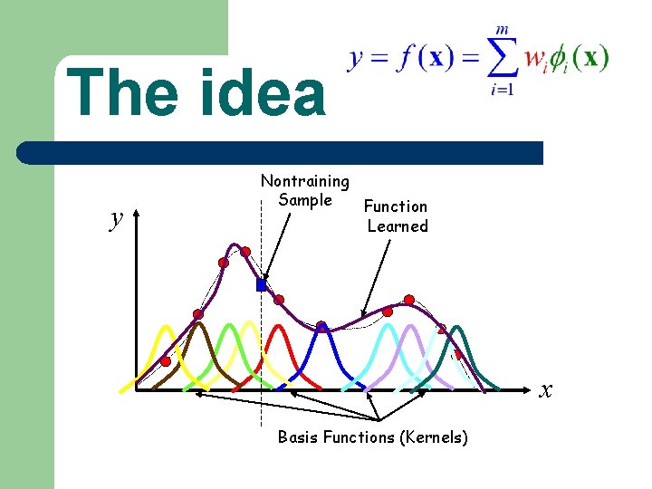
The idea y Nontraining Sample Function Learned x Basis Functions (Kernels)
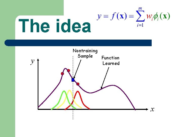
The idea y Nontraining Sample Function Learned x
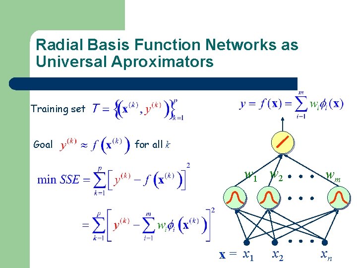
Radial Basis Function Networks as Universal Aproximators Training set Goal for all k w 1 w 2 x = x 1 x 2 wm xn
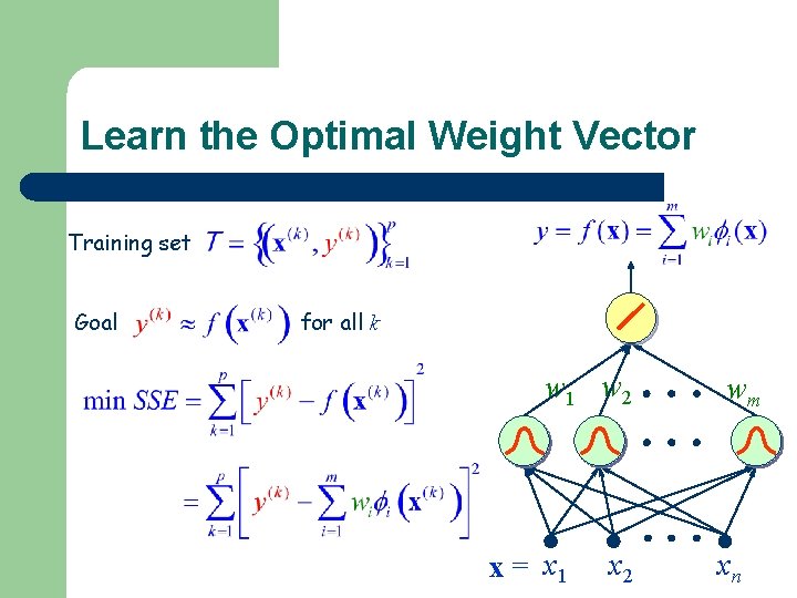
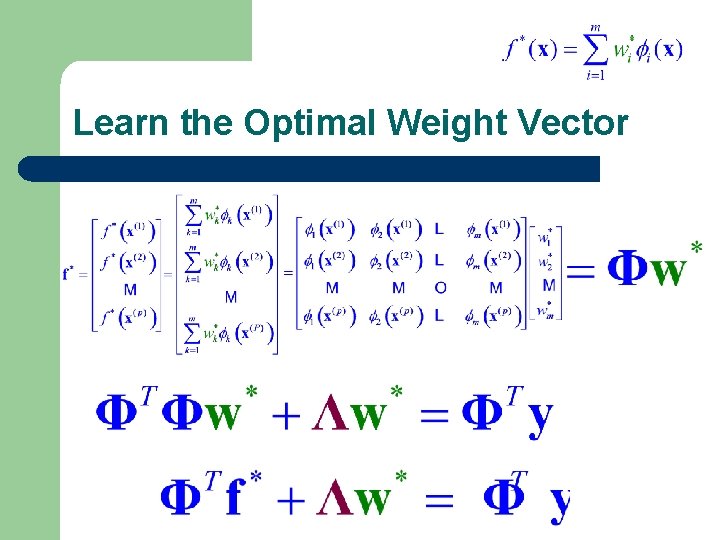
Learn the Optimal Weight Vector Training set Goal for all k w 1 w 2 x = x 1 x 2 wm xn
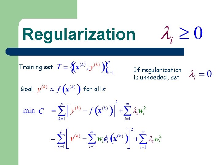
Regularization Training set Goal If regularization is unneeded, set for all k
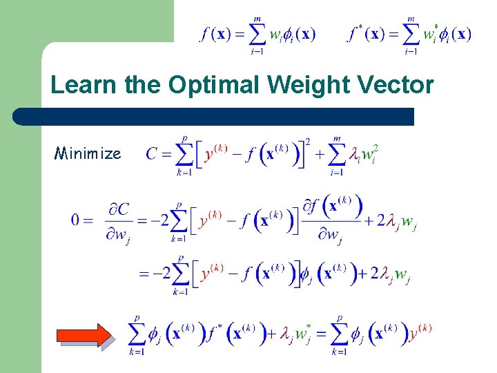
Learn the Optimal Weight Vector Minimize
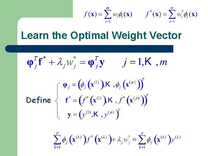
Learn the Optimal Weight Vector Define
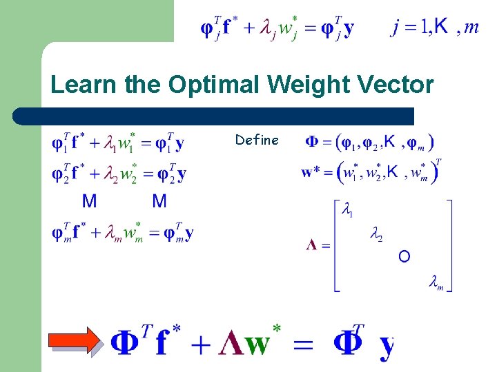
Learn the Optimal Weight Vector Define
Learn the Optimal Weight Vector
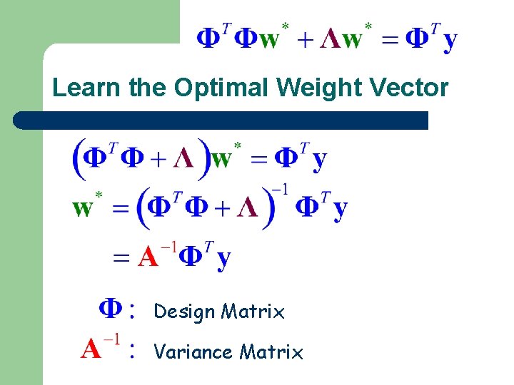
Learn the Optimal Weight Vector Design Matrix Variance Matrix
Introduction to Radial Basis Function Networks The Projection Matrix
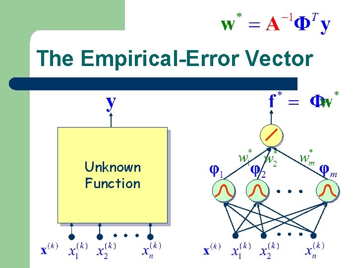
The Empirical-Error Vector Unknown Function
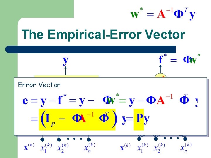
The Empirical-Error Vector Unknown Function
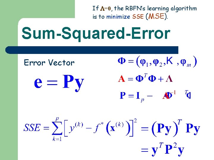
If =0, the RBFN’s learning algorithm is to minimize SSE (MSE). Sum-Squared-Error Vector
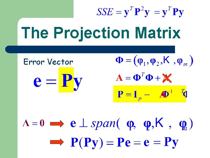
The Projection Matrix Error Vector
Introduction to Radial Basis Function Networks Learning the Kernels
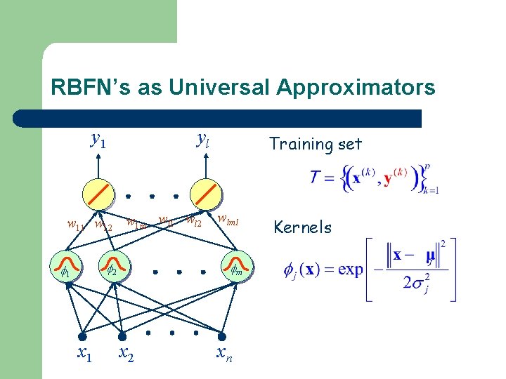
RBFN’s as Universal Approximators y 1 yl w 11 w 12 w 1 m wl 1 wl 2 2 1 x 1 Training set wlml m x 2 xn Kernels
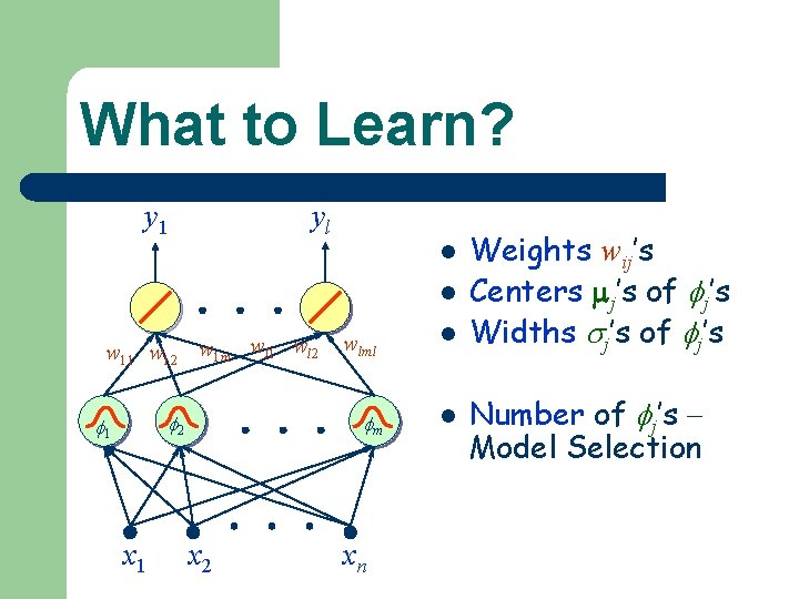
What to Learn? y 1 yl l l w 11 w 12 w 1 m wl 1 wl 2 2 1 x 2 wlml l m l xn Weights wij’s Centers j’s of j’s Widths j’s of j’s Number of j’s Model Selection
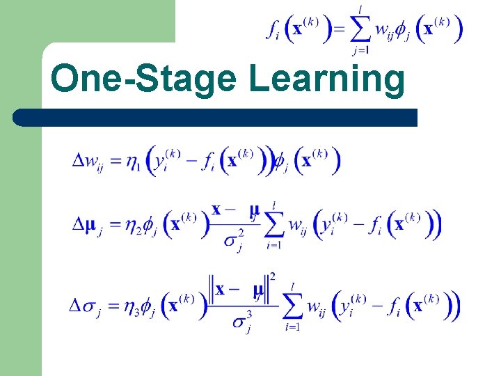
One-Stage Learning
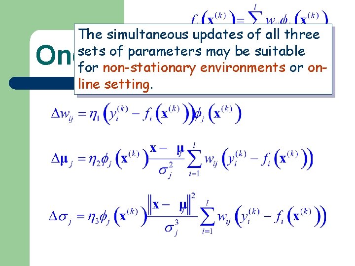
The simultaneous updates of all three sets of parameters may be suitable for non-stationary environments or online setting. One-Stage Learning
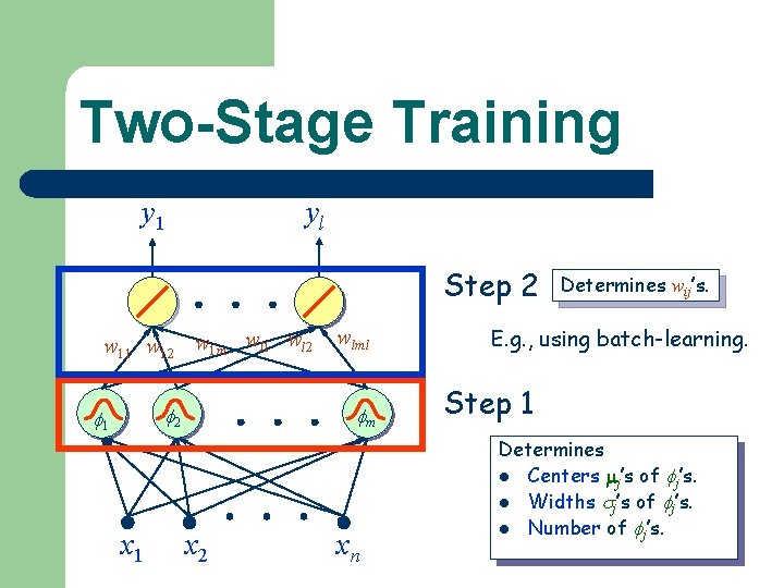
Two-Stage Training y 1 yl Step 2 w 11 w 12 w 1 m wl 1 wl 2 2 1 x 1 wlml m x 2 xn Determines wij’s. E. g. , using batch-learning. Step 1 Determines l Centers j’s of j’s. l Widths j’s of j’s. l Number of j’s.
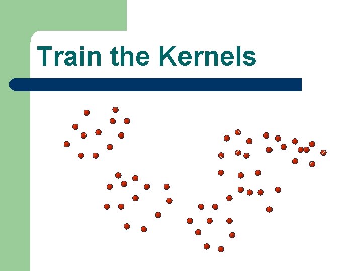
Train the Kernels
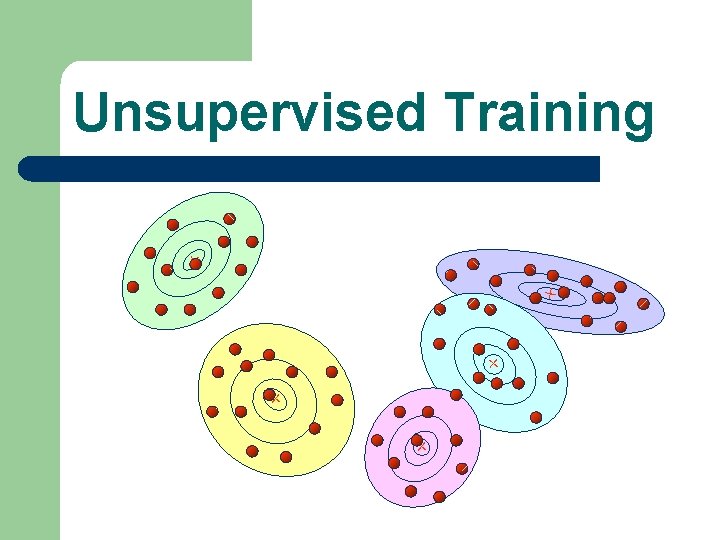
Unsupervised Training + + +
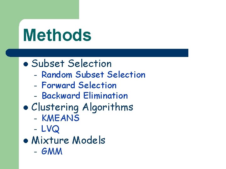
Methods l Subset Selection – – – l Clustering Algorithms – KMEANS LVQ – GMM – l Random Subset Selection Forward Selection Backward Elimination Mixture Models
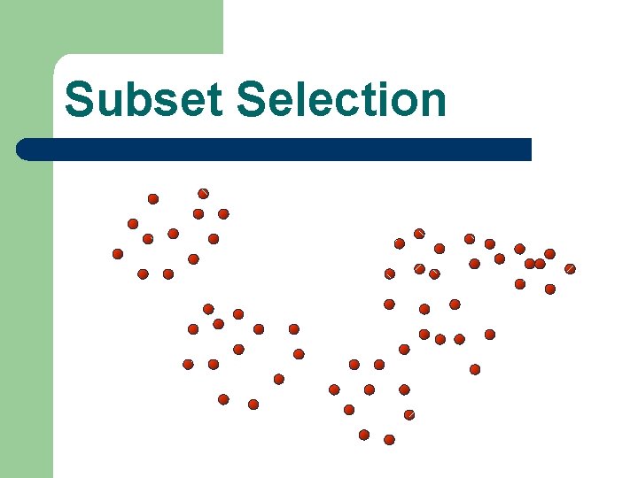
Subset Selection
Random Subset Selection l Randomly choosing a subset of points from training set l Sensitive to the initially chosen points. l Using some adaptive techniques to tune – – – Centers Widths #points
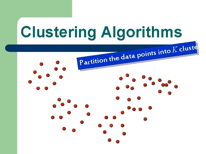
Clustering Algorithms e h t n o i t i Part rs. e t s u l c K o t n i s t n i o data p
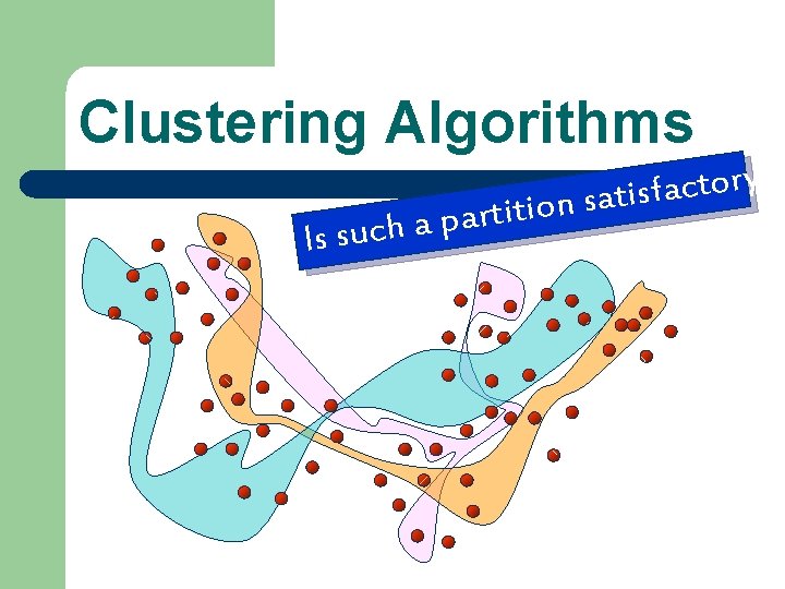
Clustering Algorithms p a h c u s Is ? y r o t c a f s i t a s n artitio
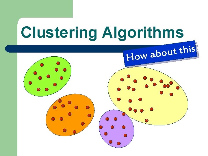
Clustering Algorithms H ? s i h t t u ow abo
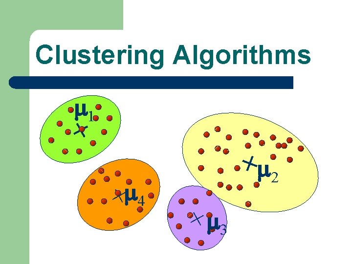
Clustering Algorithms 1 + +4 + 2 + 3
Introduction to Radial Basis Function Networks Bias-Variance Dilemma

Questions -How should the user choose the kernel? l Problem similar to that of selecting features for other learning algorithms. Ø Ø l Poor choice ---learning made very difficult. Good choice ---even poor learners could succeed. The requirement from the user is thus critical. – – can this requirement be lessened? is a more automatic selection of features possible?
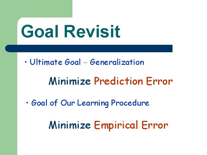
Goal Revisit • Ultimate Goal Generalization Minimize Prediction Error • Goal of Our Learning Procedure Minimize Empirical Error
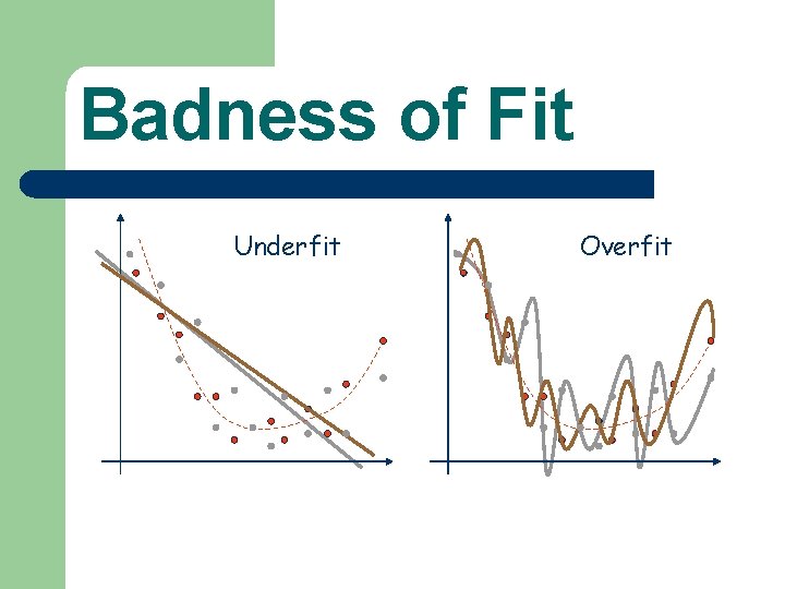
Badness of Fit l Underfitting – – l A model (e. g. , network) that is not sufficiently complex can fail to detect fully the signal in a complicated data set, leading to underfitting. Produces excessive bias in the outputs. Overfitting – – A model (e. g. , network) that is too complex may fit the noise, not just the signal, leading to overfitting. Produces excessive variance in the outputs.
Underfitting/Overfitting Avoidance l l Model selection Jittering Early stopping Weight decay – – l l Regularization Ridge Regression Bayesian learning Combining networks
Best Way to Avoid Overfitting l Use lots of training data, e. g. , – – l 30 times as many training cases as there are weights in the network. for noise-free data, 5 times as many training cases as weights may be sufficient. Don’t arbitrarily reduce the number of weights for fear of underfitting.
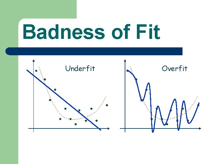
Badness of Fit Underfit Overfit
Badness of Fit Underfit Overfit
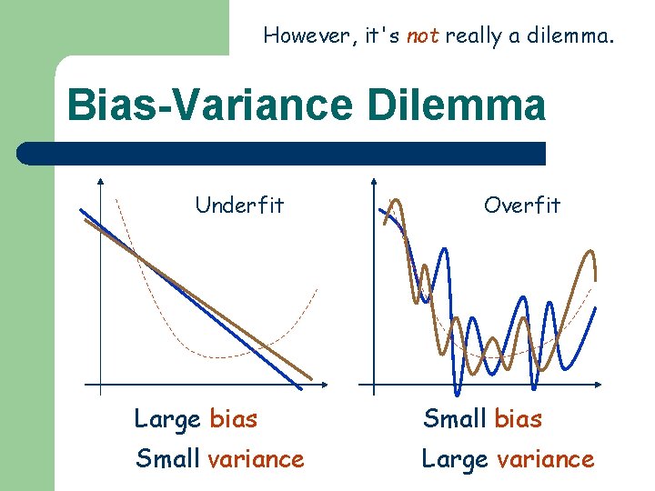
However, it's not really a dilemma. Bias-Variance Dilemma Underfit Overfit Large bias Small variance Large variance
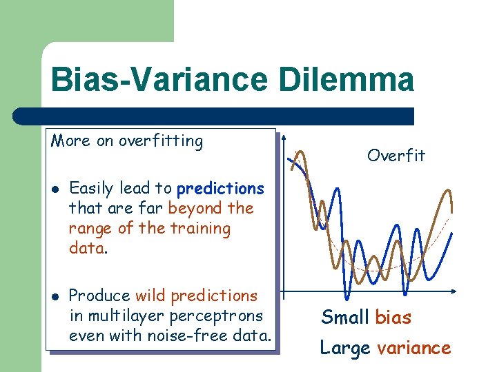
Bias-Variance Dilemma More on overfitting Underfit l l Overfit Easily lead to predictions that are far beyond the range of the training data. Produce wild predictions in multilayer perceptrons Large bias even with noise-free data. Small variance Small bias Large variance
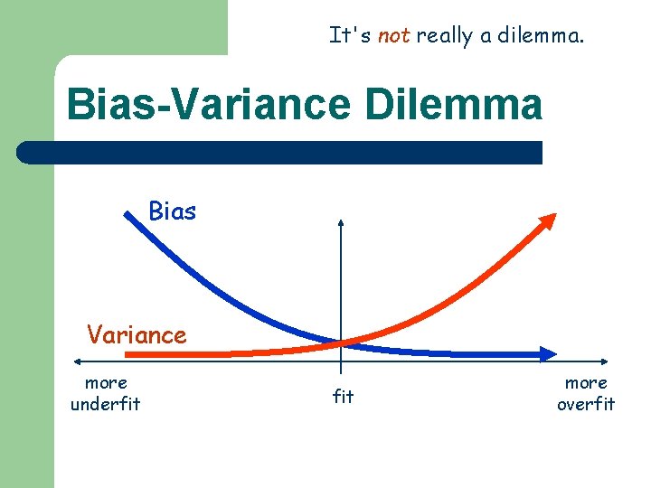
It's not really a dilemma. Bias-Variance Dilemma Bias Variance more underfit more overfit
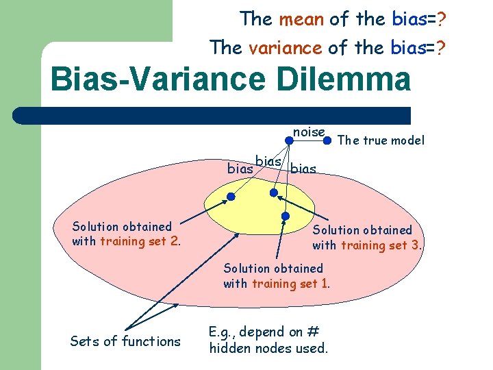
The mean of the bias=? The variance of the bias=? Bias-Variance Dilemma noise bias Solution obtained with training set 2. bias Solution obtained with training set 3. Solution obtained with training set 1. Sets of functions The true model E. g. , depend on # hidden nodes used.
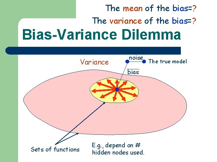
The mean of the bias=? The variance of the bias=? Bias-Variance Dilemma Variance noise bias Sets of functions E. g. , depend on # hidden nodes used. The true model
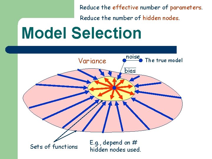
Reduce the effective number of parameters. Reduce the number of hidden nodes. Model Selection Variance noise bias Sets of functions E. g. , depend on # hidden nodes used. The true model
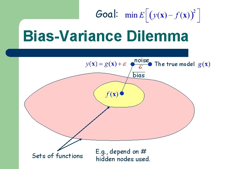
Goal: Bias-Variance Dilemma noise bias Sets of functions E. g. , depend on # hidden nodes used. The true model
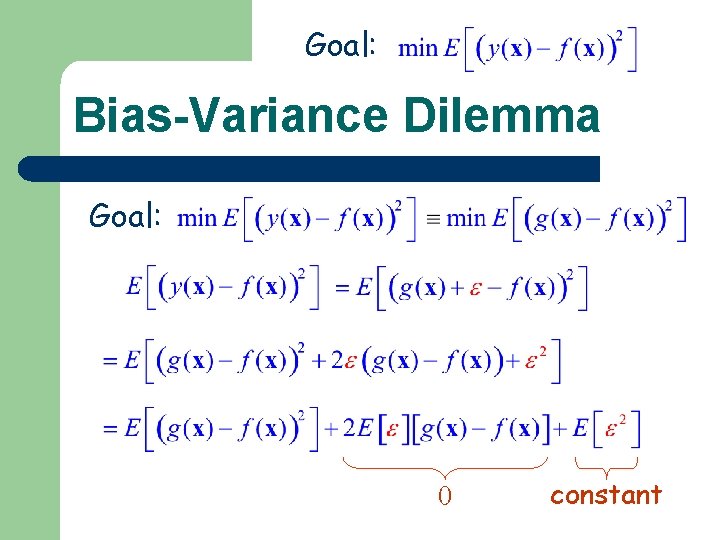
Goal: Bias-Variance Dilemma Goal: 0 constant
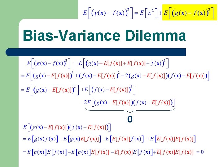
Bias-Variance Dilemma 0
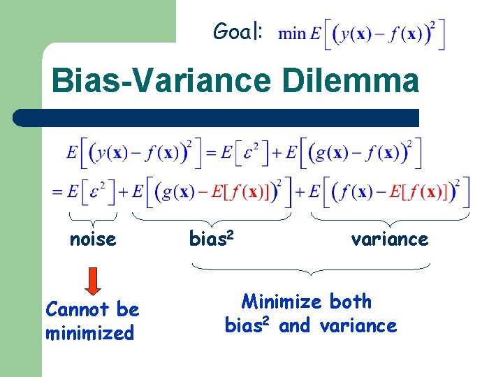
Goal: Bias-Variance Dilemma noise Cannot be minimized bias 2 variance Minimize both bias 2 and variance
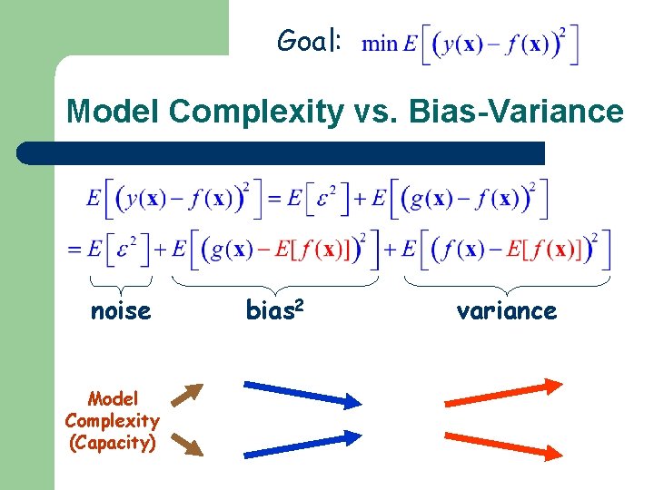
Goal: Model Complexity vs. Bias-Variance noise Model Complexity (Capacity) bias 2 variance
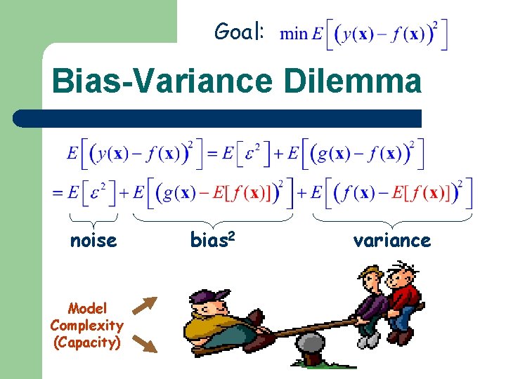
Goal: Bias-Variance Dilemma noise Model Complexity (Capacity) bias 2 variance
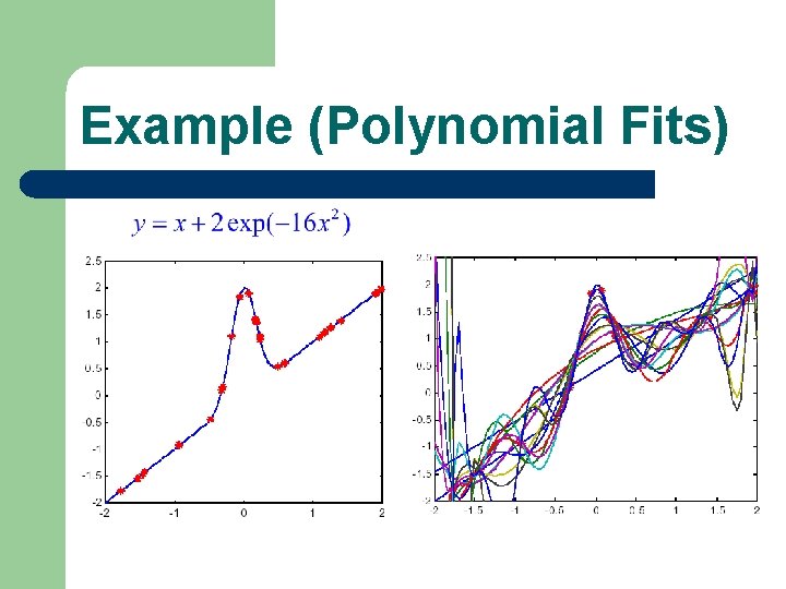
Example (Polynomial Fits)
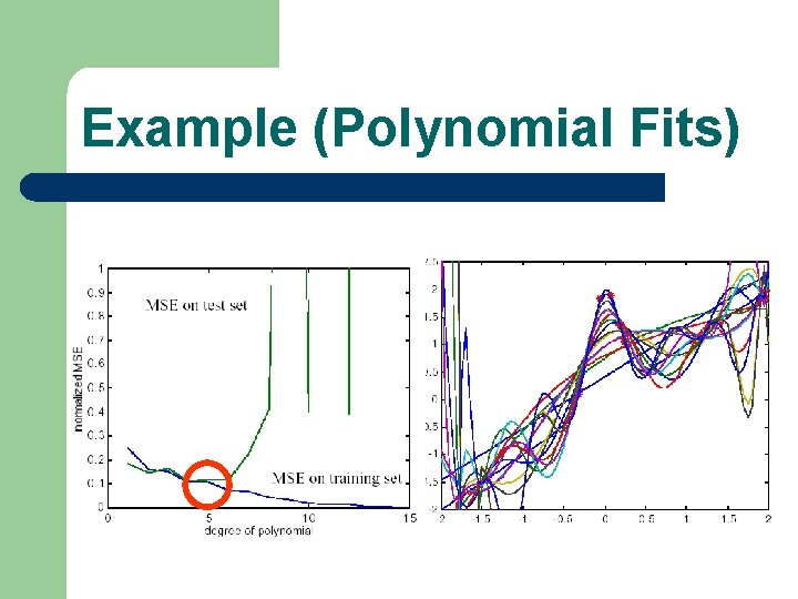
Example (Polynomial Fits)
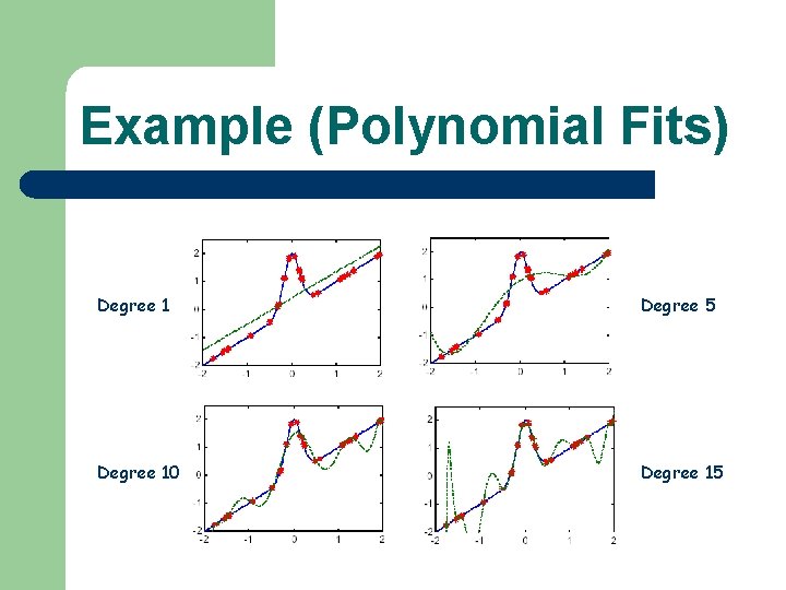
Example (Polynomial Fits) Degree 1 Degree 5 Degree 10 Degree 15
Introduction to Radial Basis Function Networks The Effective Number of Parameters
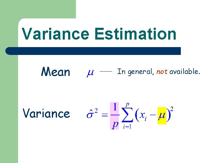
Variance Estimation Mean Variance In general, not available.
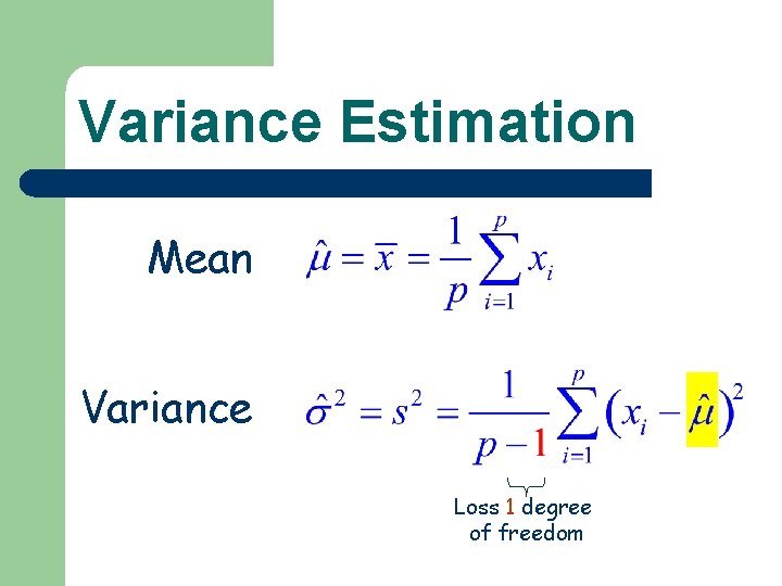
Variance Estimation Mean Variance Loss 1 degree of freedom
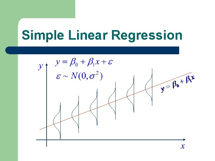
Simple Linear Regression
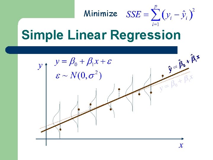
Minimize Simple Linear Regression
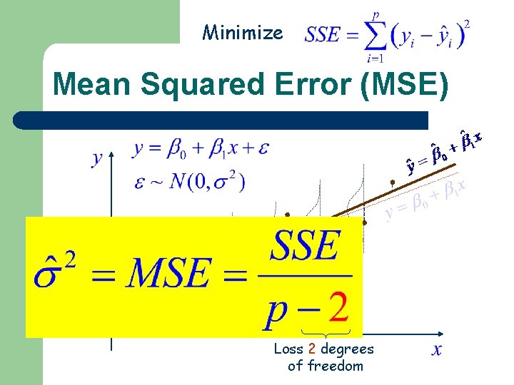
Minimize Mean Squared Error (MSE) Loss 2 degrees of freedom
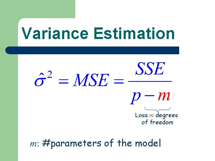
Variance Estimation Loss m degrees of freedom m: #parameters of the model
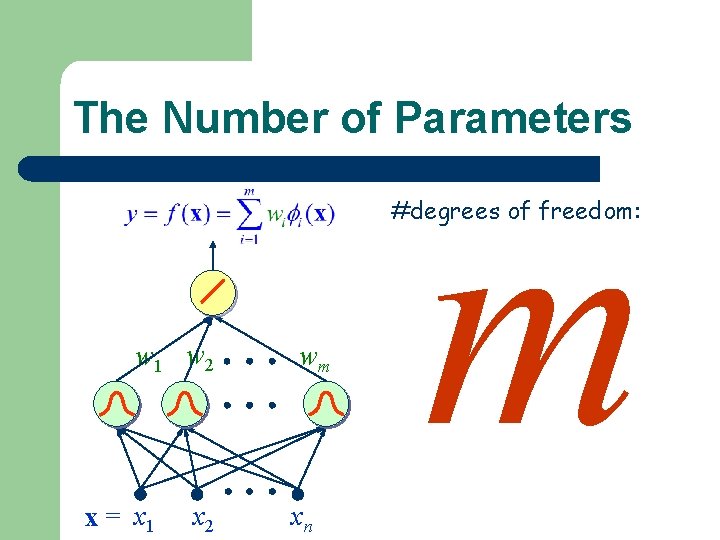
The Number of Parameters m #degrees of freedom: w 1 w 2 x = x 1 x 2 wm xn
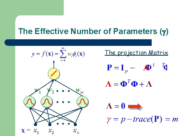
The Effective Number of Parameters ( ) The projection Matrix w 1 w 2 x = x 1 x 2 wm xn
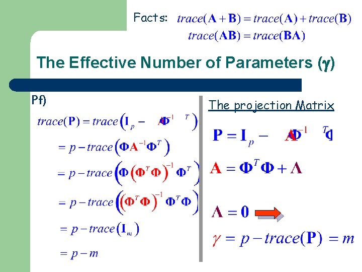
Facts: The Effective Number of Parameters ( ) Pf) The projection Matrix
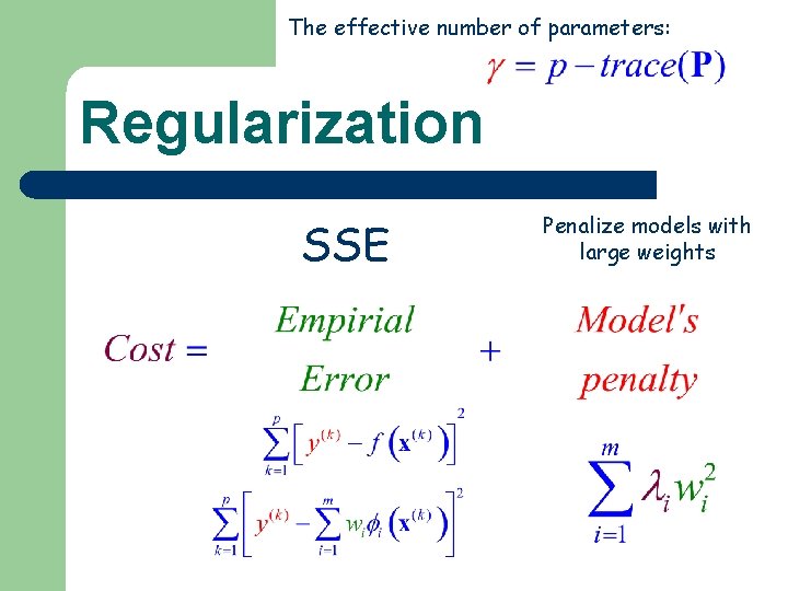
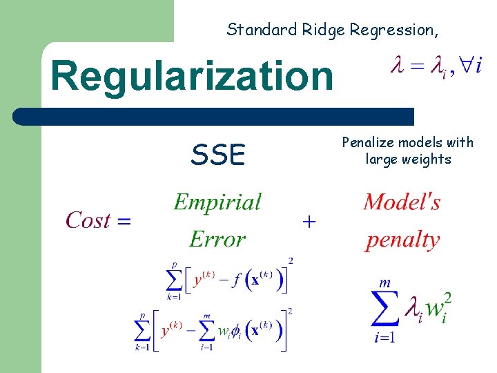
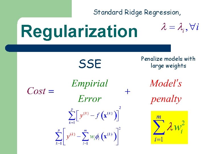
The effective number of parameters: Regularization SSE Penalize models with large weights
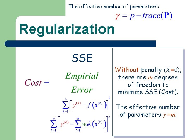
The effective number of parameters: Regularization SSE Penalize models with large weights Without penalty ( i=0), there are m degrees of freedom to minimize SSE (Cost). The effective number of parameters =m.
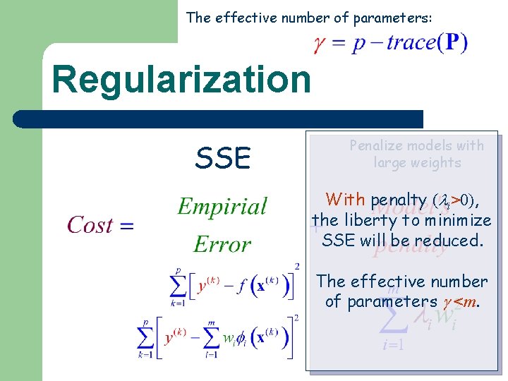
The effective number of parameters: Regularization SSE Penalize models with large weights With penalty ( i>0), the liberty to minimize SSE will be reduced. The effective number of parameters <m.
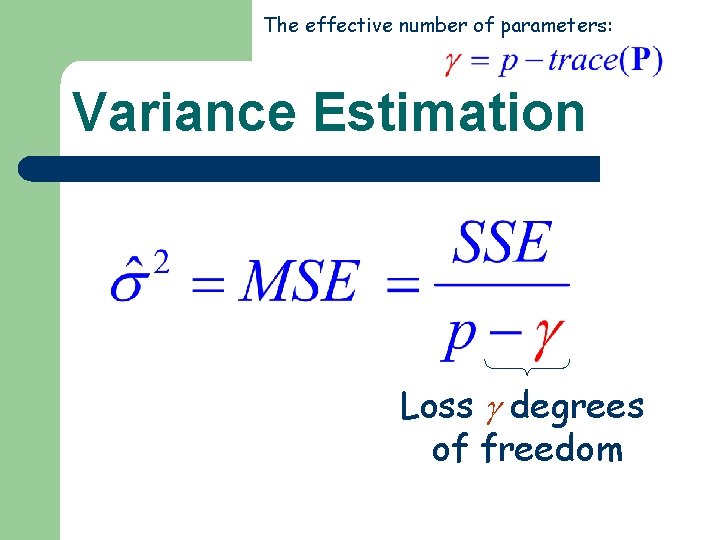
The effective number of parameters: Variance Estimation Loss degrees of freedom
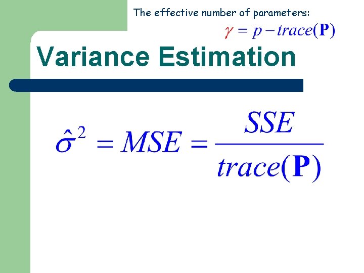
The effective number of parameters: Variance Estimation

Introduction to Radial Basis Function Networks Model Selection
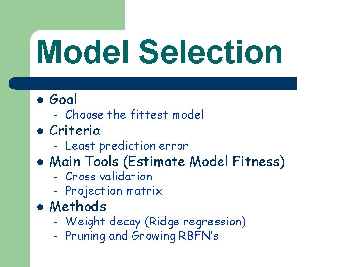
Model Selection l l l Goal – Choose the fittest model – Least prediction error – Cross validation Projection matrix Criteria Main Tools (Estimate Model Fitness) – l Methods – – Weight decay (Ridge regression) Pruning and Growing RBFN’s
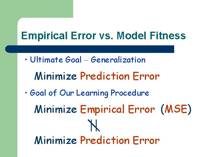
Empirical Error vs. Model Fitness • Ultimate Goal Generalization Minimize Prediction Error • Goal of Our Learning Procedure Minimize Empirical Error (MSE) Minimize Prediction Error
Estimating Prediction Error l When you have plenty of data use independent test sets – l E. g. , use the same training set to train different models, and choose the best model by comparing on the test set. When data is scarce, use – – Cross-Validation Bootstrap
Cross Validation l l Simplest and most widely used method for estimating prediction error. Partition the original set into several different ways and to compute an average score over the different partitions, e. g. , – – – K-fold Cross-Validation Leave-One-Out Cross-Validation Generalize Cross-Validation
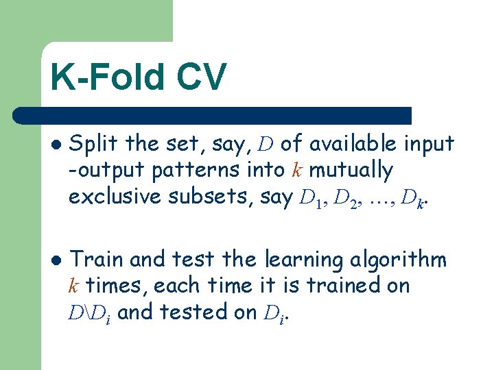
K-Fold CV l l Split the set, say, D of available input -output patterns into k mutually exclusive subsets, say D 1, D 2, …, Dk. Train and test the learning algorithm k times, each time it is trained on DDi and tested on Di.

K-Fold CV Available Data
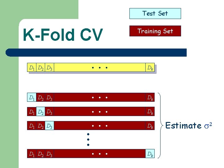
Test Set K-Fold CV D 1 D 2 D 3 . . . Available Data D 1 D 2 D 3 . . . D 1 D 2 D 3 Training Set Dk Dk Dk Estimate 2
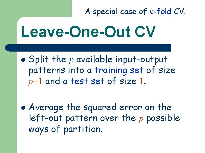
A special case of k-fold CV. Leave-One-Out CV l l Split the p available input-output patterns into a training set of size p 1 and a test set of size 1. Average the squared error on the left-out pattern over the p possible ways of partition.
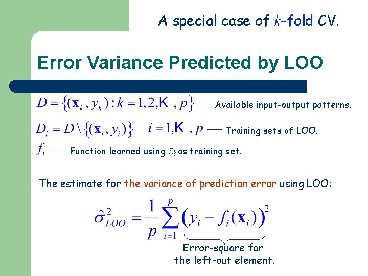
A special case of k-fold CV. Error Variance Predicted by LOO Available input-output patterns. Training sets of LOO. Function learned using Di as training set. The estimate for the variance of prediction error using LOO: Error-square for the left-out element.
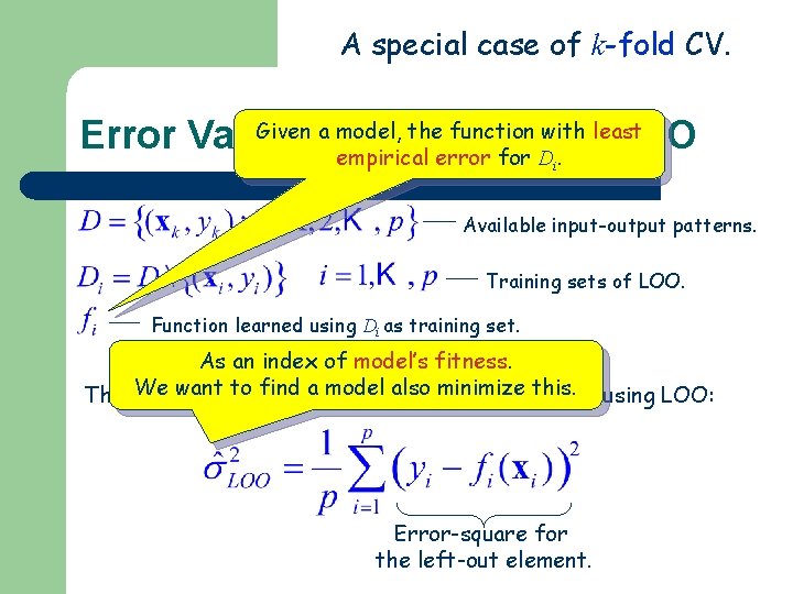
A special case of k-fold CV. Given a model, the function with least Error Variance Predicted by LOO empirical error for D. i Available input-output patterns. Training sets of LOO. Function learned using Di as training set. As an index of model’s fitness. We want for to find model also minimize this. The estimate the avariance of prediction error using LOO: Error-square for the left-out element.
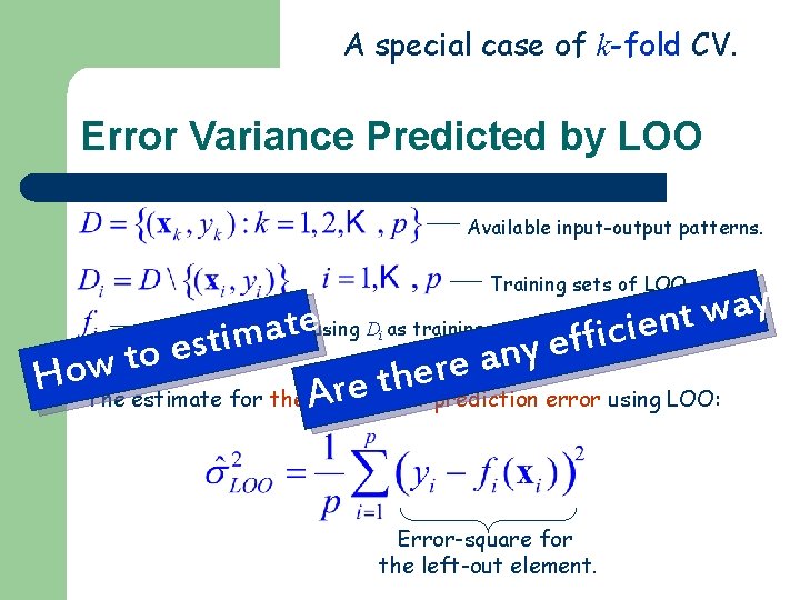
A special case of k-fold CV. Error Variance Predicted by LOO Available input-output patterns. Training sets of LOO. ? s y a w t n e i c i f f e ? e t a m i t s e y n o t a e w r e Ho. The h t re of prediction error using LOO: estimate for the A variance Function learned using Di as training set. Error-square for the left-out element.
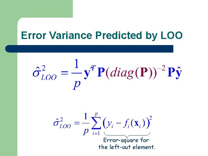
Error Variance Predicted by LOO Error-square for the left-out element.
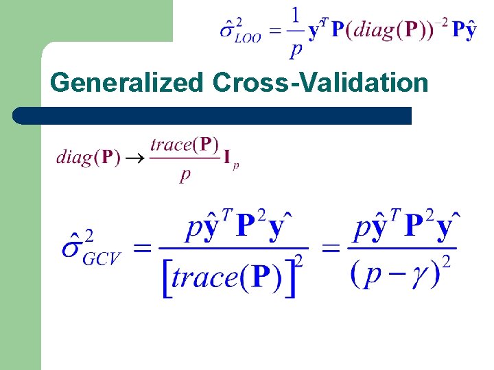
Generalized Cross-Validation
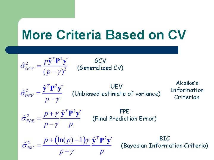
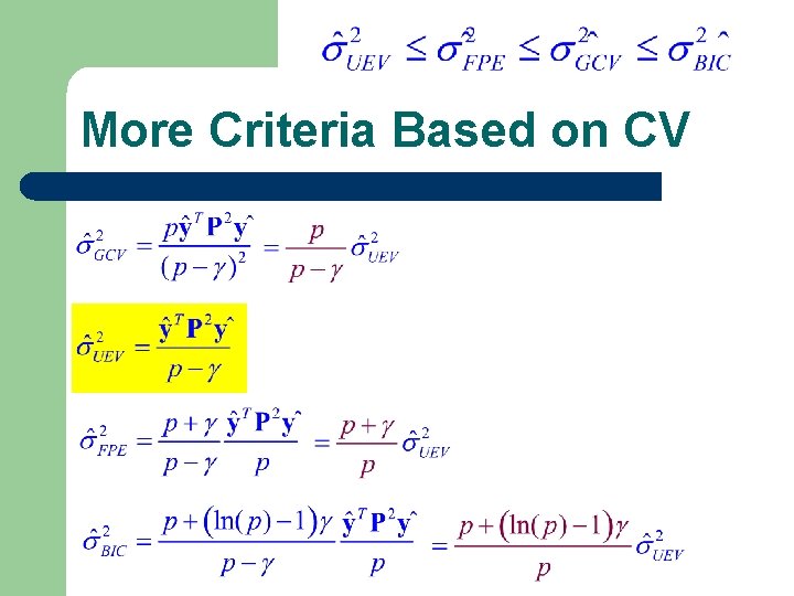
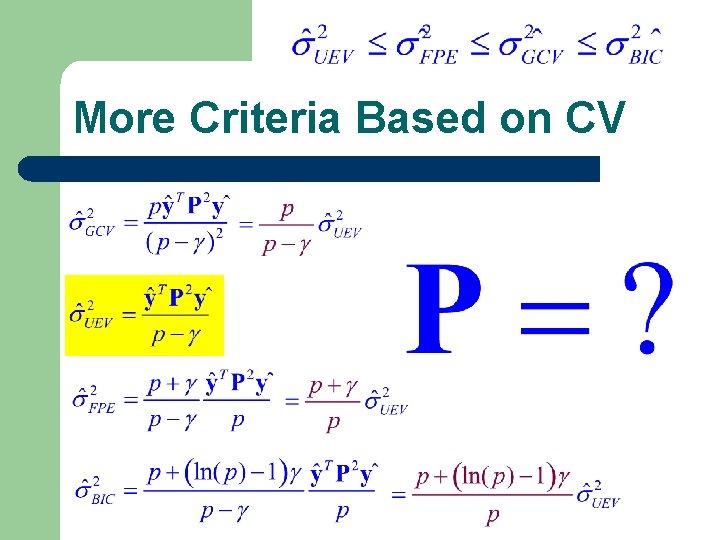
More Criteria Based on CV GCV (Generalized CV) UEV (Unbiased estimate of variance) Akaike’s Information Criterion FPE (Final Prediction Error) BIC (Bayesian Information Criterio)
More Criteria Based on CV
More Criteria Based on CV
Standard Ridge Regression, Regularization SSE Penalize models with large weights
Standard Ridge Regression, Regularization SSE Penalize models with large weights
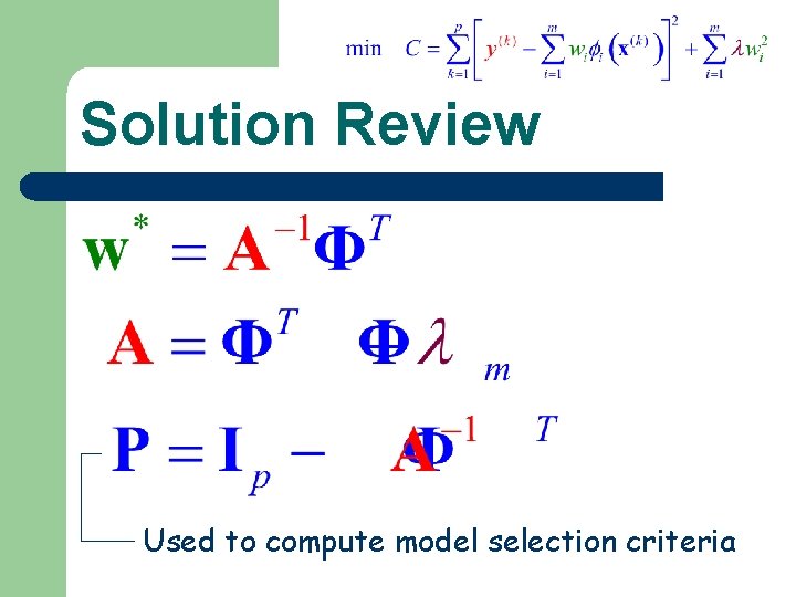
Solution Review Used to compute model selection criteria
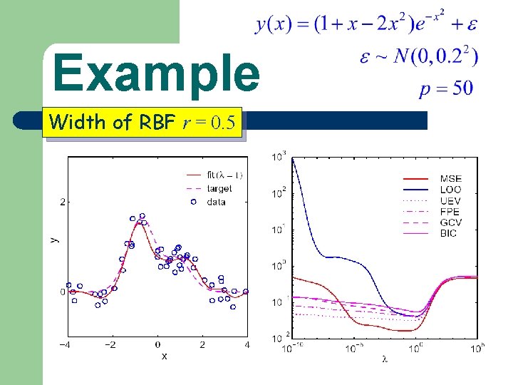
Example Width of RBF r = 0. 5
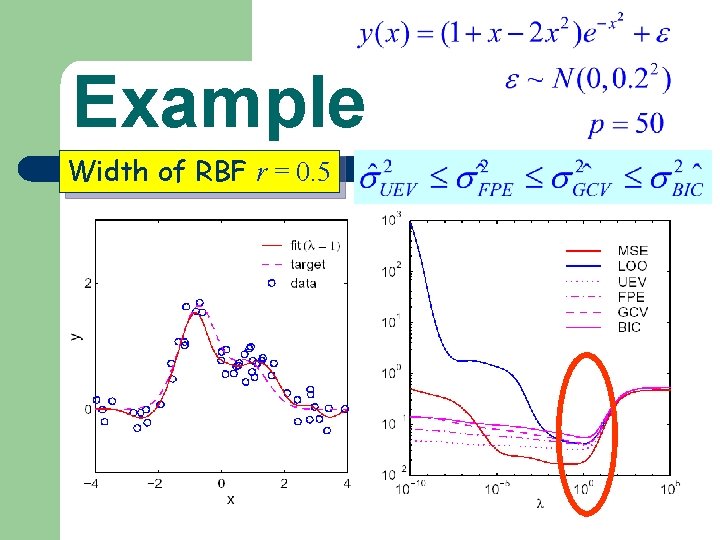
Example Width of RBF r = 0. 5
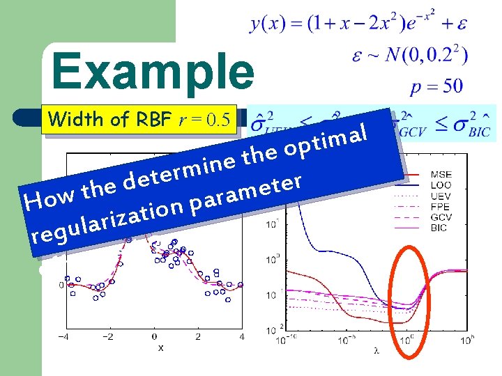
Example Width of RBF r = 0. 5 l a m i t p o e h t e n i m r e t e r d e t e e h t m a w r o a p H n o i t a z i r a l regu ? y l e v i t c e f ef
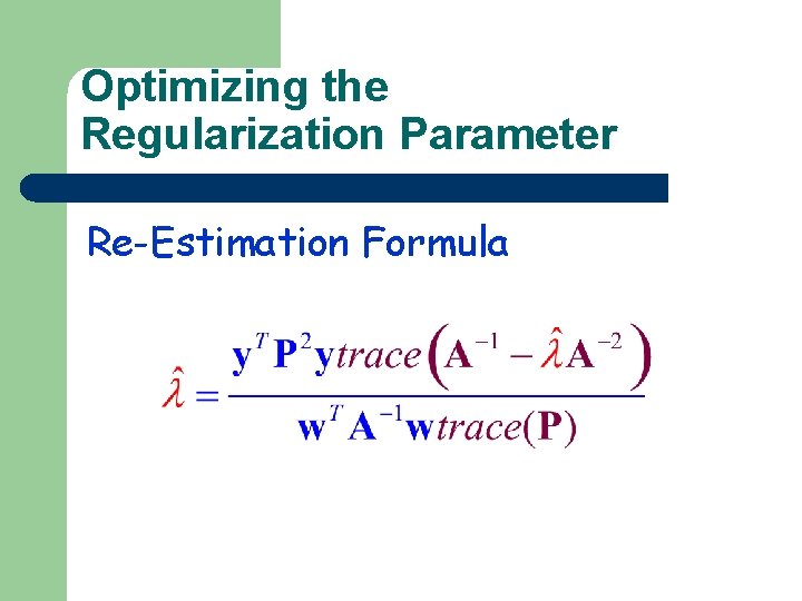
Optimizing the Regularization Parameter Re-Estimation Formula
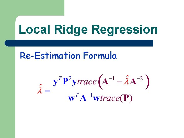
Local Ridge Regression Re-Estimation Formula
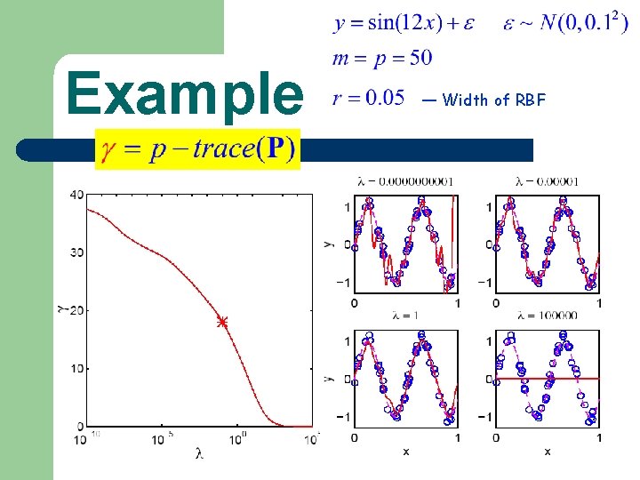
Example — Width of RBF
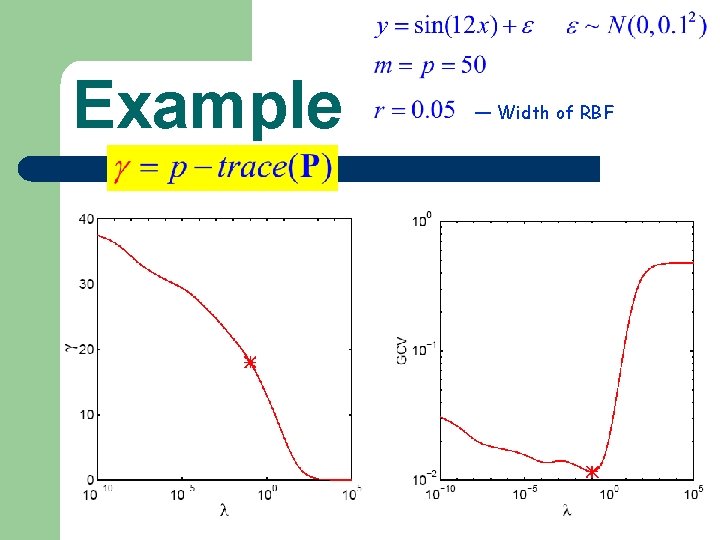
Example — Width of RBF
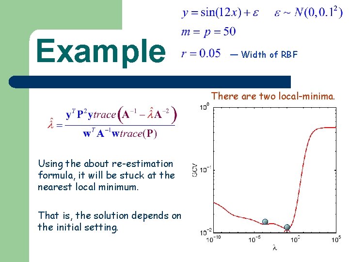
Example — Width of RBF There are two local-minima. Using the about re-estimation formula, it will be stuck at the nearest local minimum. That is, the solution depends on the initial setting.
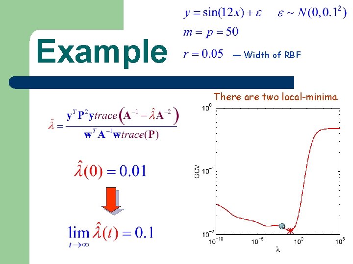
Example — Width of RBF There are two local-minima.
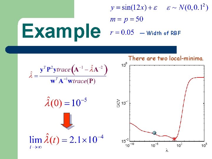
Example — Width of RBF There are two local-minima.
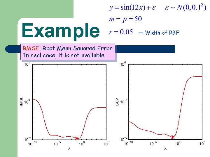
Example RMSE: Root Mean Squared Error In real case, it is not available. — Width of RBF
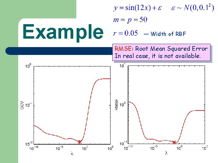
Example — Width of RBF RMSE: Root Mean Squared Error In real case, it is not available.
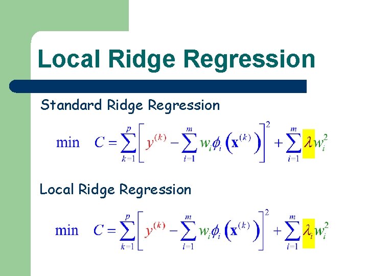
Local Ridge Regression Standard Ridge Regression Local Ridge Regression
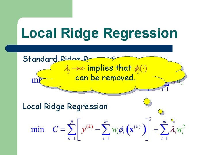
Local Ridge Regression Standard Ridge Regression j implies that j( ) can be removed. Local Ridge Regression
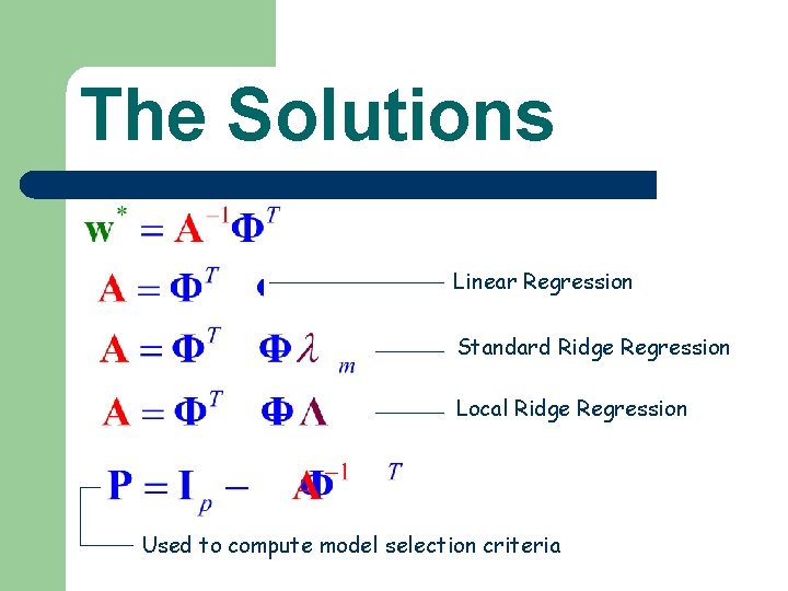
The Solutions Linear Regression Standard Ridge Regression Local Ridge Regression Used to compute model selection criteria
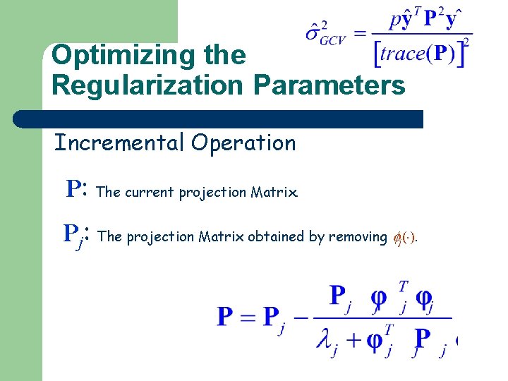
Optimizing the Regularization Parameters Incremental Operation P: The current projection Matrix. Pj: The projection Matrix obtained by removing ( ). j
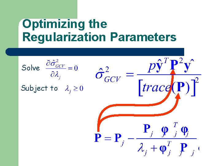
Optimizing the Regularization Parameters Solve Subject to
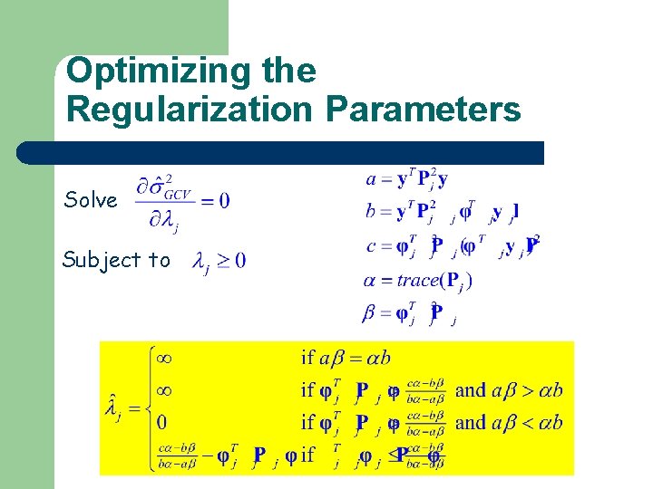
Optimizing the Regularization Parameters Solve Subject to
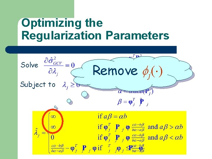
Optimizing the Regularization Parameters Solve Subject to Remove j( )
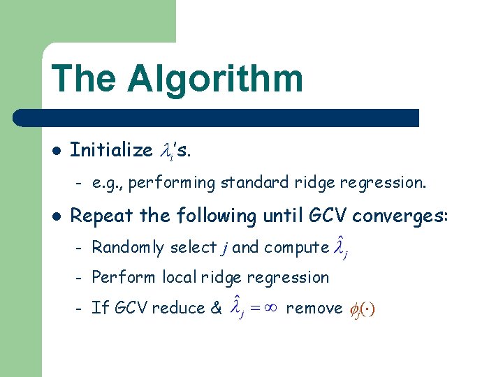
The Algorithm l Initialize i’s. – l e. g. , performing standard ridge regression. Repeat the following until GCV converges: – Randomly select j and compute – Perform local ridge regression – If GCV reduce & remove j( )
- Slides: 136