Introduction to R with Tidyverse Simon Andrews v

Introduction to R (with Tidyverse) Simon Andrews v 2020 -07

R can just be a calculator > 3+2 [1] 5 > 2/7 [1] 0. 2857143 > 5^10 [1] 9765625

Storing numerical data in variables 10 -> x y <- 20 x [1] 10 x+y [1] 30 x+y -> z

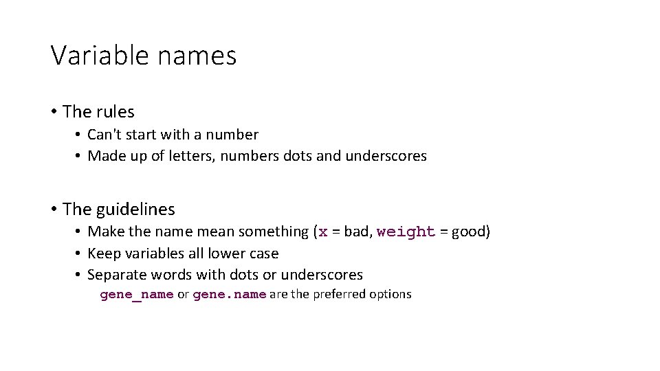
Variable names • The rules • Can't start with a number • Made up of letters, numbers dots and underscores • The guidelines • Make the name mean something (x = bad, weight = good) • Keep variables all lower case • Separate words with dots or underscores gene_name or gene. name are the preferred options

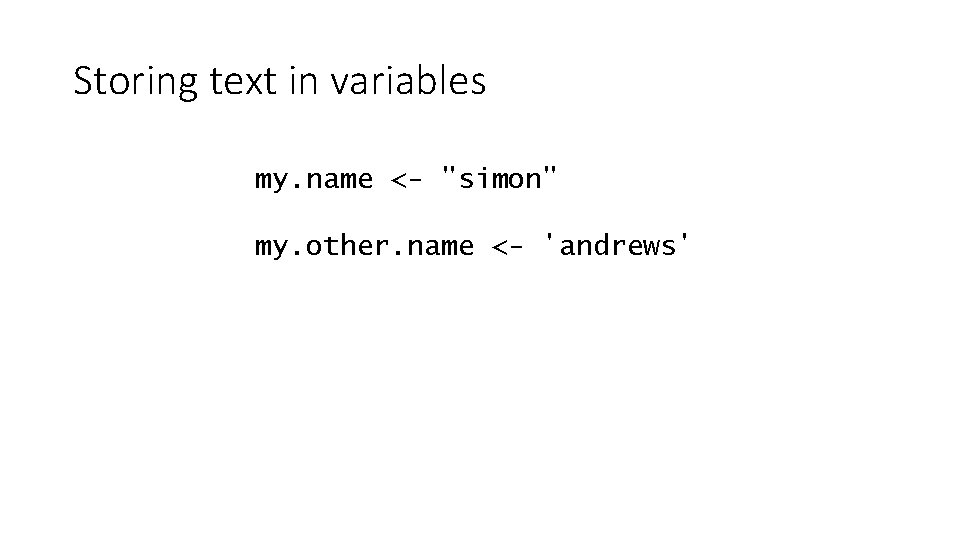
Storing text in variables my. name <- "simon" my. other. name <- 'andrews'

Running a simple function sqrt(10) [1] 3. 162278

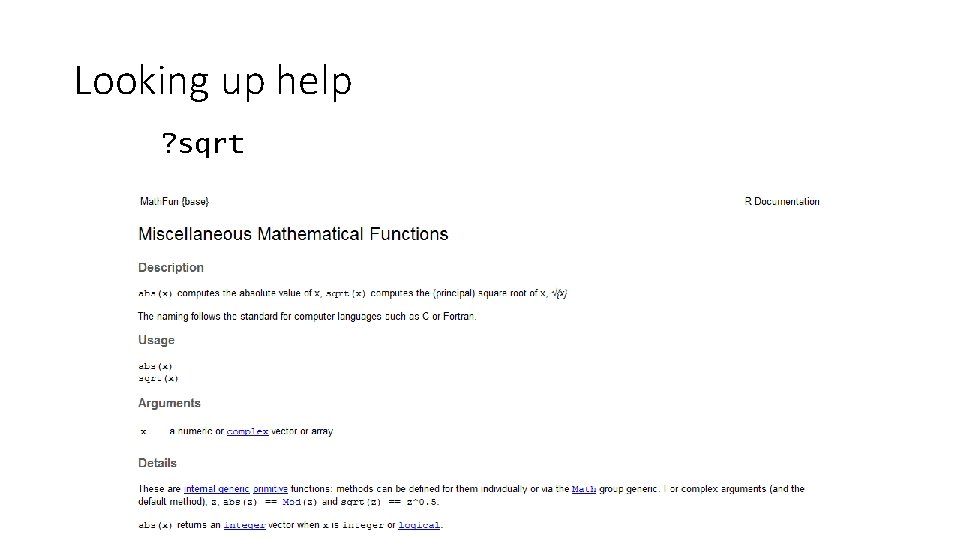
Looking up help ? sqrt

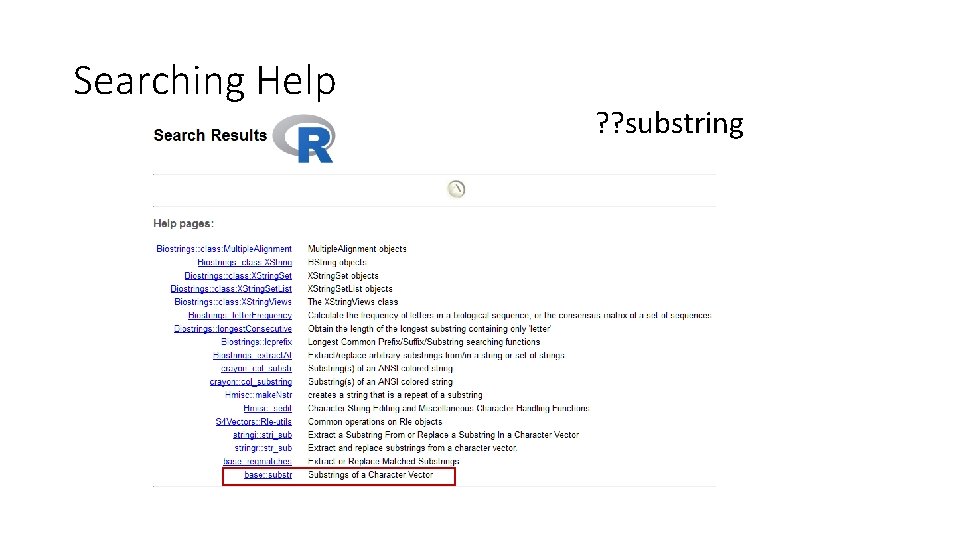
Searching Help ? ? substring

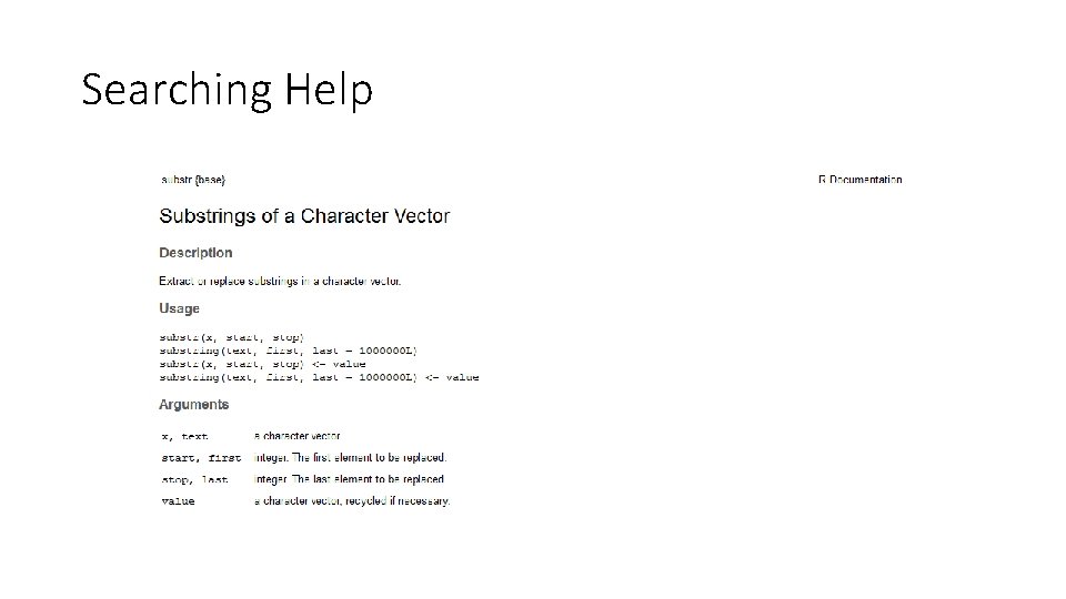
Searching Help

Passing arguments to functions substr(my. name, 2, 4) [1] "imo" substr(x=my. name, start=2, stop=4) [1] "imo" substr( start=2, stop=4, x=my. name ) [1] "imo"

Exercise 1

Everything is a vector • Vectors are the most basic unit of storage in R • Vectors are ordered sets of values of the same type • • • Numeric Character (text) Factor (repeated text values) Logical (TRUE or FALSE) Date etc… 10 -> x x is a vector of length 1 with 10 as its first value

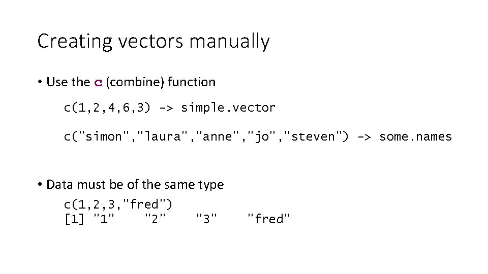
Creating vectors manually • Use the c (combine) function c(1, 2, 4, 6, 3) -> simple. vector c("simon", "laura", "anne", "jo", "steven") -> some. names • Data must be of the same type c(1, 2, 3, "fred") [1] "1" "2" "3" "fred"

Functions for creating vectors • rep - repeat values rep(2, times=10) [1] 2 2 2 2 2 rep("hello", times=5) [1] "hello" "hello" rep(c("dog", "cat"), times=3) [1] "dog" "cat" rep(c("dog", "cat"), each=3) [1] "dog" "cat"

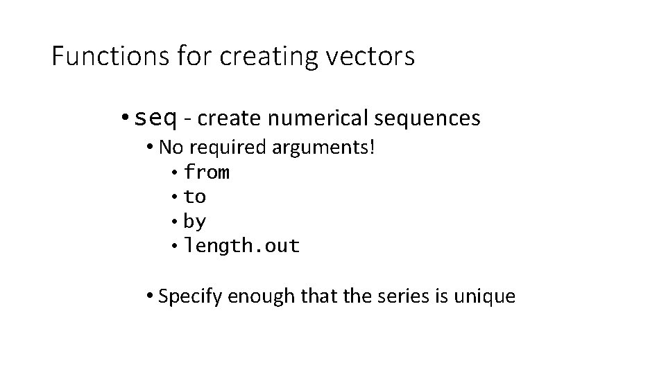
Functions for creating vectors • seq - create numerical sequences • No required arguments! • from • to • by • length. out • Specify enough that the series is unique

Functions for creating vectors • seq - create numerical sequences seq(from=2, by=3, to=14) [1] 2 5 8 11 14 seq(from=3, by=10, to=40) [1] 3 13 23 33 seq(from=5, by=3. 6, length. out=5) [1] 5. 0 8. 6 12. 2 15. 8 19. 4

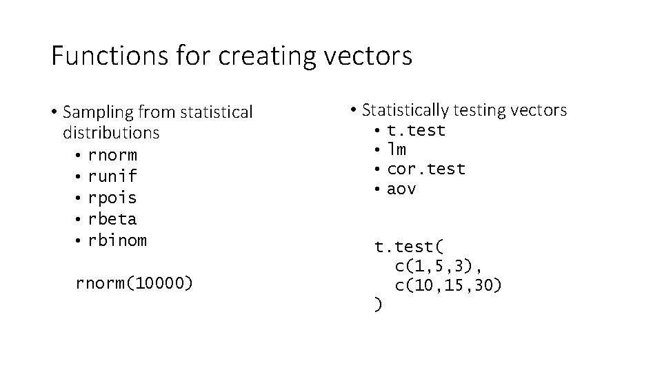
Functions for creating vectors • Sampling from statistical distributions • • • rnorm runif rpois rbeta rbinom rnorm(10000) • Statistically testing vectors • • t. test lm cor. test aov t. test( c(1, 5, 3), c(10, 15, 30) )

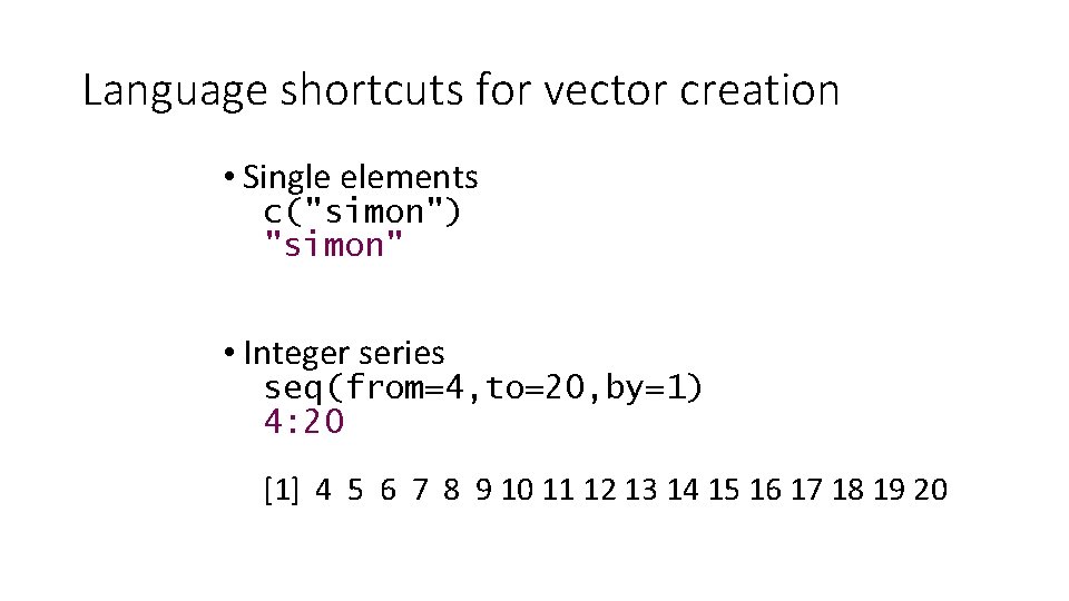
Language shortcuts for vector creation • Single elements c("simon") "simon" • Integer series seq(from=4, to=20, by=1) 4: 20 [1] 4 5 6 7 8 9 10 11 12 13 14 15 16 17 18 19 20

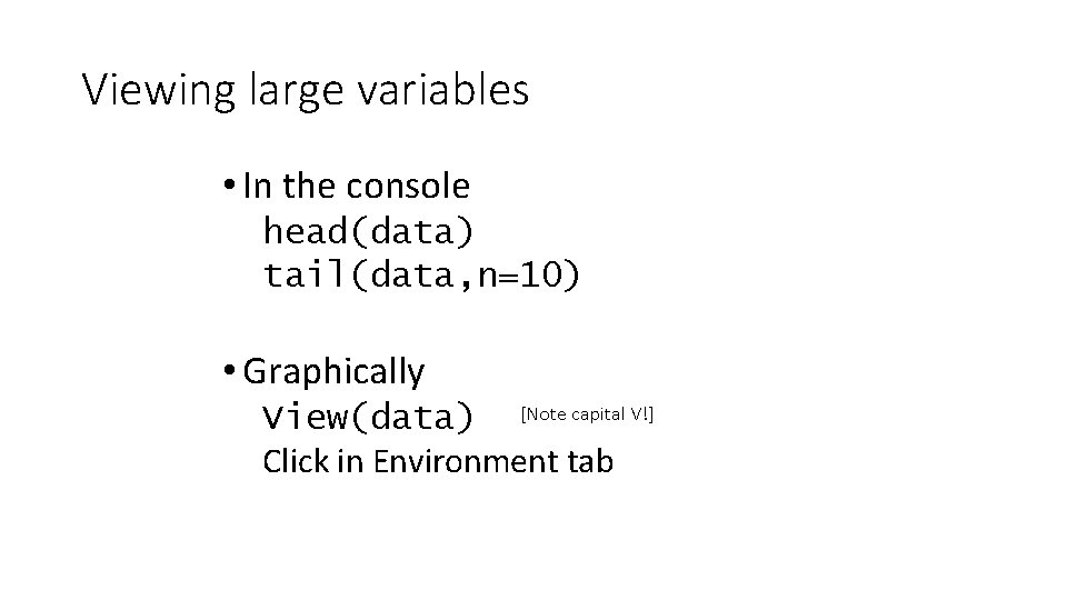
Viewing large variables • In the console head(data) tail(data, n=10) • Graphically View(data) [Note capital V!] Click in Environment tab

Vectorised Operations 2+3 [1] 5 c(2, 4) + c(3, 5) [1] 5 9 simple. vector 1 2 4 6 3 simple. vector * 100 200 400 600 300

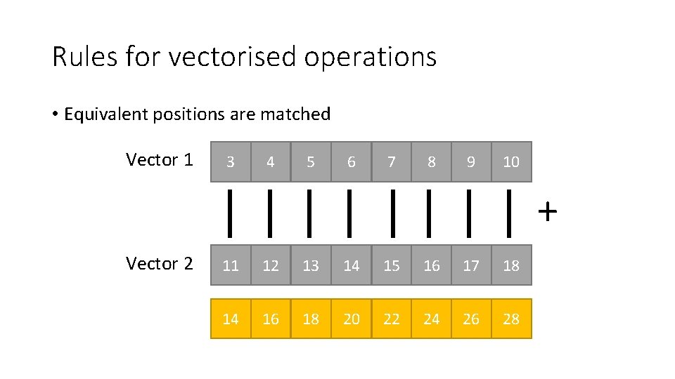
Rules for vectorised operations • Equivalent positions are matched Vector 1 3 4 5 6 7 8 9 10 + Vector 2 11 12 13 14 15 16 17 18 14 16 18 20 22 24 26 28

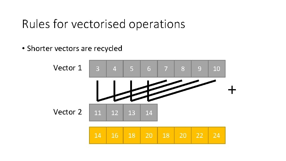
Rules for vectorised operations • Shorter vectors are recycled Vector 1 3 4 5 6 7 8 9 10 + Vector 2 11 12 13 14 14 16 18 20 22 24

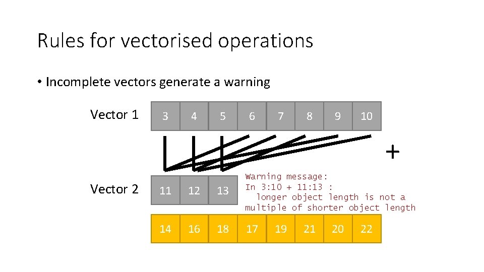
Rules for vectorised operations • Incomplete vectors generate a warning Vector 1 3 4 5 6 7 8 9 10 + Vector 2 11 12 13 Warning message: In 3: 10 + 11: 13 : longer object length is not a multiple of shorter object length 14 16 18 17 19 21 20 22

Vectorised Operations c(2, 4) + c(3, 5) [1] 5 9 simple. vector 1 2 4 6 3 simple. vector * 100 200 400 600 300

Exercise 2

R Data Structures

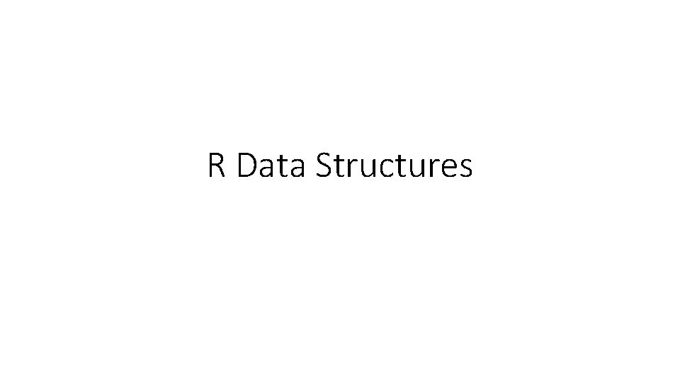
Vector • 1 D Data Structure of fixed type scores 1 0. 8 2 1. 2 3 3. 3 4 1. 8 5 2. 7 mean(scores) sd(scores)

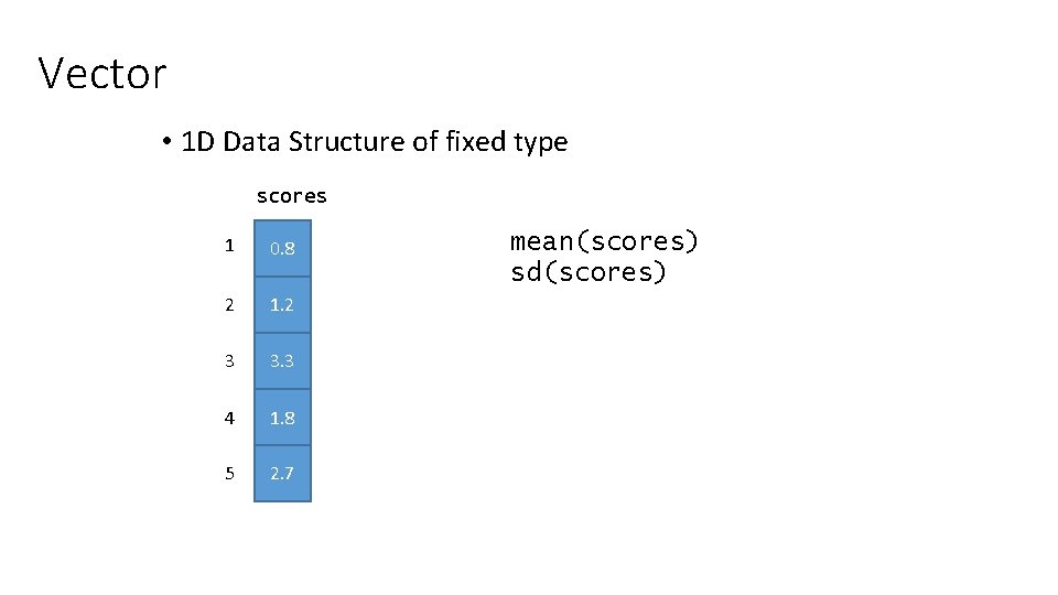
List • Collection of vectors results$counts mean(results$counts) results “ratios” 1 “counts” 2 1 0. 8 1 100 2 1. 2 2 300 3 3 200 4 1. 8 5 2. 7

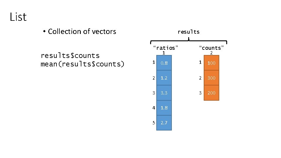
Data Frame • Collection of vectors with same lengths • Gain the concept of 'rows' all. results$mon mean(all. results$mon) all. results “tue” “wed” “pass” 1 2 3 4 1 0. 8 0. 9 0. 8 T 2 0. 6 0. 7 0. 5 F 3 0. 2 0. 3 F 4 0. 8 0. 9 T 5 0. 6 1. 0 0. 9 T “mon”

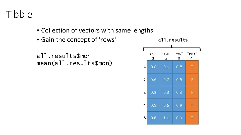
Tibble • Collection of vectors with same lengths • Gain the concept of 'rows' all. results$mon mean(all. results$mon) all. results “tue” “wed” “pass” 1 2 3 4 1 0. 8 0. 9 0. 8 T 2 0. 6 0. 7 0. 5 F 3 0. 2 0. 3 F 4 0. 8 0. 9 T 5 0. 6 1. 0 0. 9 T “mon”

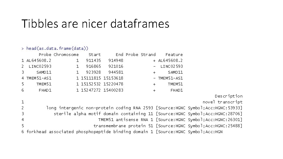
Tibbles are nicer dataframes > head(as. data. frame(data)) Probe Chromosome Start End Probe Strand Feature 1 AL 645608. 2 1 911435 914948 + AL 645608. 2 2 LINC 02593 1 916865 921016 - LINC 02593 3 SAMD 11 1 923928 944581 + SAMD 11 4 TMEM 51 -AS 1 1 15111815 15153618 - TMEM 51 -AS 1 5 TMEM 51 1 15152532 15220478 + TMEM 51 6 FHAD 1 1 15247272 15400283 + FHAD 1 1 2 long intergenic non-protein coding RNA 2593 3 sterile alpha motif domain containing 11 4 TMEM 51 antisense RNA 1 5 transmembrane protein 51 6 forkhead associated phosphopeptide binding domain 1 [Source: HGNC [Source: HGNC Description novel transcript Symbol; Acc: HGNC: 53933] Symbol; Acc: HGNC: 28706] Symbol; Acc: HGNC: 26301] Symbol; Acc: HGNC: 25488] Symbol; Acc: HGN

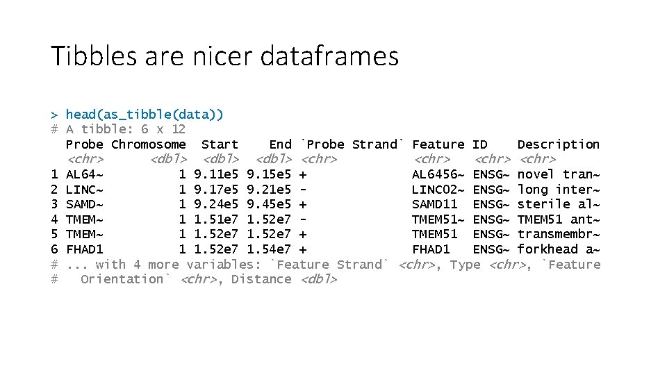
Tibbles are nicer dataframes > head(as_tibble(data)) # A tibble: 6 x 12 Probe Chromosome Start <chr> 1 2 3 4 5 6 # # <dbl> End `Probe Strand` Feature ID <dbl> <chr> Description <chr> AL 64~ 1 9. 11 e 5 9. 15 e 5 + AL 6456~ ENSG~ novel tran~ LINC~ 1 9. 17 e 5 9. 21 e 5 LINC 02~ ENSG~ long inter~ SAMD~ 1 9. 24 e 5 9. 45 e 5 + SAMD 11 ENSG~ sterile al~ TMEM~ 1 1. 51 e 7 1. 52 e 7 TMEM 51~ ENSG~ TMEM 51 ant~ TMEM~ 1 1. 52 e 7 + TMEM 51 ENSG~ transmembr~ FHAD 1 1 1. 52 e 7 1. 54 e 7 + FHAD 1 ENSG~ forkhead a~. . . with 4 more variables: `Feature Strand` <chr>, Type <chr>, `Feature Orientation` <chr>, Distance <dbl>

Tidyverse https: //www. tidyverse. org/ • Collection of R packages • Aims to fix many of core R's structural problems • Common design and data philosophy • Designed to work together, but integrate seamlessly with other parts of R

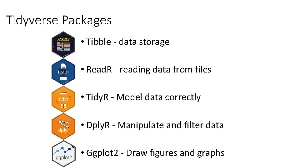
Tidyverse Packages • Tibble - data storage • Read. R - reading data from files • Tidy. R - Model data correctly • Dply. R - Manipulate and filter data • Ggplot 2 - Draw figures and graphs

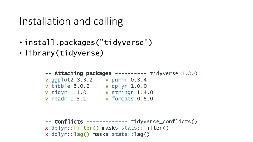
Installation and calling • install. packages("tidyverse") • library(tidyverse) -- Attaching packages ----- tidyverse 1. 3. 0 – v ggplot 2 3. 3. 2 v purrr 0. 3. 4 v tibble 3. 0. 2 v dplyr 1. 0. 0 v tidyr 1. 1. 0 v stringr 1. 4. 0 v readr 1. 3. 1 v forcats 0. 5. 0 -- Conflicts ------- tidyverse_conflicts() – x dplyr: : filter() masks stats: : filter() x dplyr: : lag() masks stats: : lag()

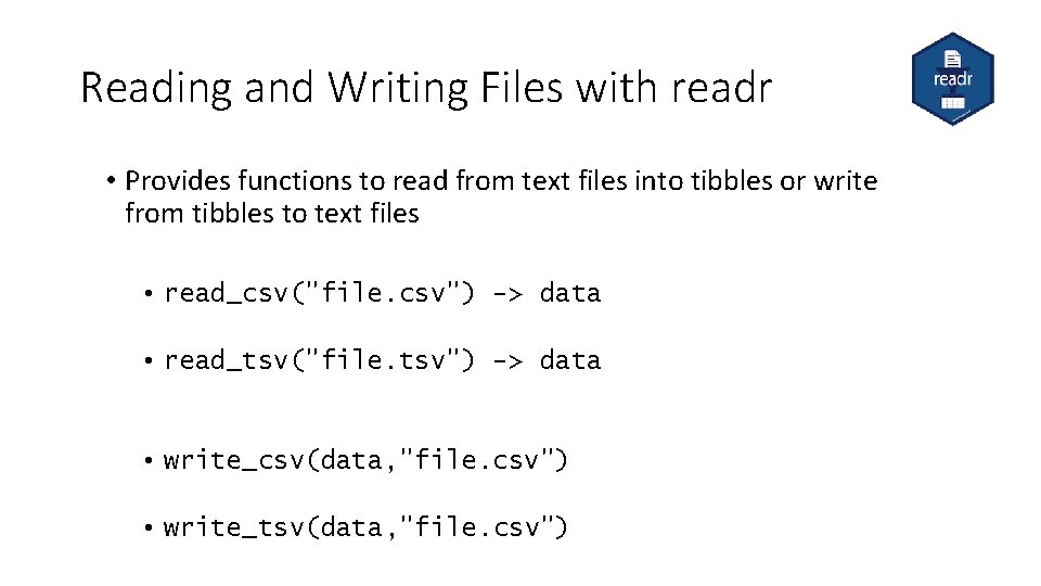
Reading and Writing Files with readr • Provides functions to read from text files into tibbles or write from tibbles to text files • read_csv("file. csv") -> data • read_tsv("file. tsv") -> data • write_csv(data, "file. csv") • write_tsv(data, "file. csv")

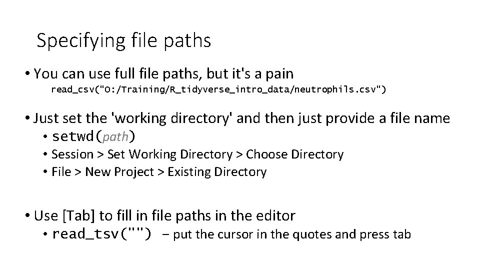
Specifying file paths • You can use full file paths, but it's a pain read_csv("O: /Training/R_tidyverse_intro_data/neutrophils. csv") • Just set the 'working directory' and then just provide a file name • setwd(path) • Session > Set Working Directory > Choose Directory • File > New Project > Existing Directory • Use [Tab] to fill in file paths in the editor • read_tsv("") – put the cursor in the quotes and press tab

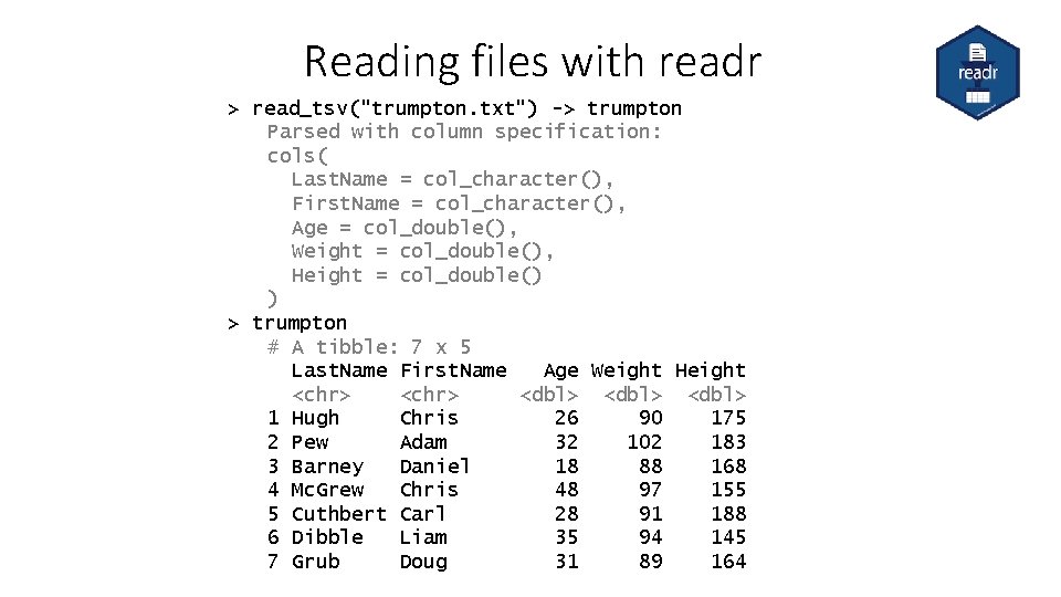
Reading files with readr > read_tsv("trumpton. txt") -> trumpton Parsed with column specification: cols( Last. Name = col_character(), First. Name = col_character(), Age = col_double(), Weight = col_double(), Height = col_double() ) > trumpton # A tibble: 7 x 5 Last. Name First. Name Age Weight Height <chr> <dbl> 1 Hugh Chris 26 90 175 2 Pew Adam 32 102 183 3 Barney Daniel 18 88 168 4 Mc. Grew Chris 48 97 155 5 Cuthbert Carl 28 91 188 6 Dibble Liam 35 94 145 7 Grub Doug 31 89 164

Exercise 3

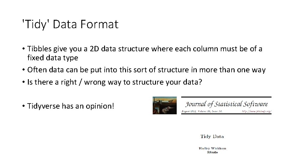
'Tidy' Data Format • Tibbles give you a 2 D data structure where each column must be of a fixed data type • Often data can be put into this sort of structure in more than one way • Is there a right / wrong way to structure your data? • Tidyverse has an opinion!

Long vs Wide Data Modelling • Consider a simple experiment: • Two genes tested (ABC 1 and DEF 1) • Two conditions (WT and KO) • Three replicates for each condition

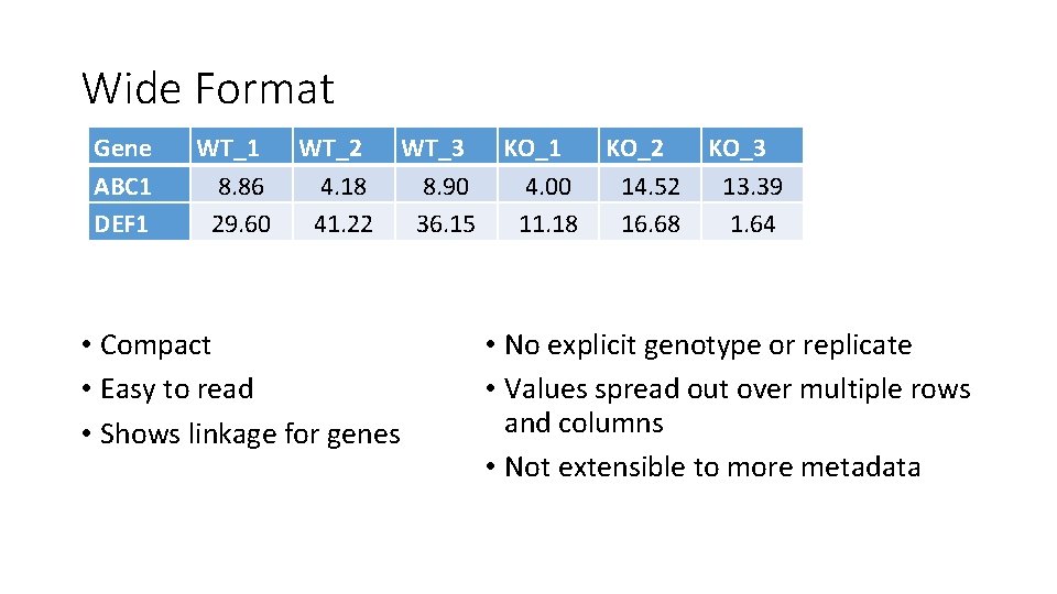
Wide Format Gene ABC 1 DEF 1 WT_1 8. 86 29. 60 WT_2 4. 18 41. 22 • Compact • Easy to read • Shows linkage for genes WT_3 8. 90 36. 15 KO_1 4. 00 11. 18 KO_2 14. 52 16. 68 KO_3 13. 39 1. 64 • No explicit genotype or replicate • Values spread out over multiple rows and columns • Not extensible to more metadata

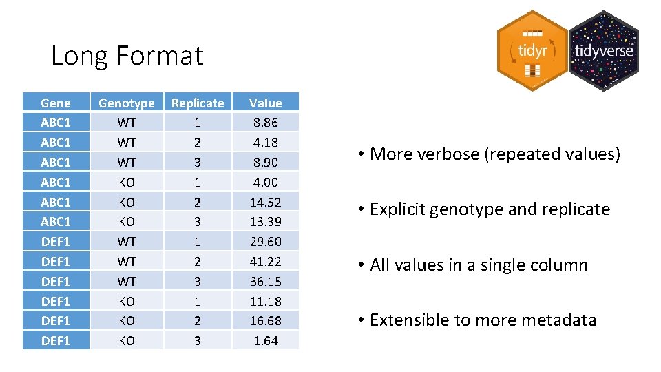
Long Format Gene ABC 1 ABC 1 DEF 1 DEF 1 Genotype WT WT WT KO KO KO Replicate 1 2 3 Value 8. 86 4. 18 8. 90 4. 00 14. 52 13. 39 29. 60 41. 22 36. 15 11. 18 16. 68 1. 64 • More verbose (repeated values) • Explicit genotype and replicate • All values in a single column • Extensible to more metadata

Filtering and subsetting • Tidyverse (specifically dplyr) comes with functions to manipulate your data. • All functions take a tibble as their first argument • All functions return a modified tibble • Selecting columns • Logical subsetting

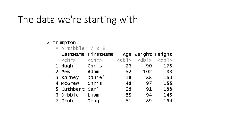
The data we're starting with > trumpton # A tibble: 7 x 5 Last. Name First. Name Age Weight Height <chr> <dbl> 1 Hugh Chris 26 90 175 2 Pew Adam 32 102 183 3 Barney Daniel 18 88 168 4 Mc. Grew Chris 48 97 155 5 Cuthbert Carl 28 91 188 6 Dibble Liam 35 94 145 7 Grub Doug 31 89 164

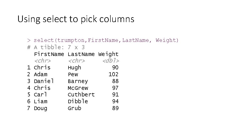
Using select to pick columns > select(trumpton, First. Name, Last. Name, Weight) # A tibble: 7 x 3 First. Name Last. Name Weight 1 2 3 4 5 6 7 <chr> Chris Adam Daniel Chris Carl Liam Doug Hugh Pew Barney Mc. Grew Cuthbert Dibble Grub <dbl> 90 102 88 97 91 94 89

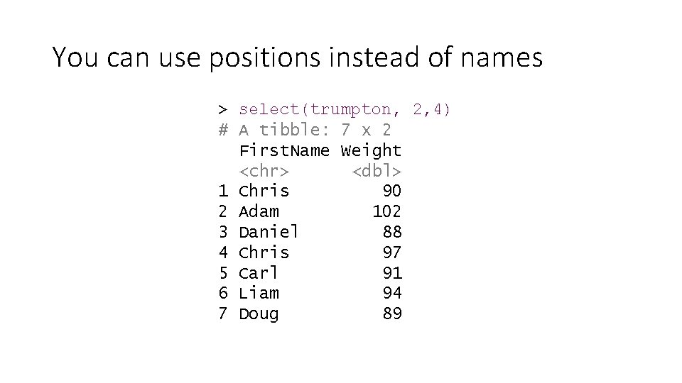
You can use positions instead of names > select(trumpton, 2, 4) # A tibble: 7 x 2 First. Name Weight <chr> <dbl> 1 Chris 90 2 Adam 102 3 Daniel 88 4 Chris 97 5 Carl 91 6 Liam 94 7 Doug 89

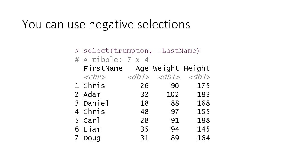
You can use negative selections > select(trumpton, -Last. Name) # A tibble: 7 x 4 First. Name Age Weight Height <chr> 1 2 3 4 5 6 7 Chris Adam Daniel Chris Carl Liam Doug <dbl> 26 32 18 48 28 35 31 90 102 88 97 91 94 89 175 183 168 155 188 145 164

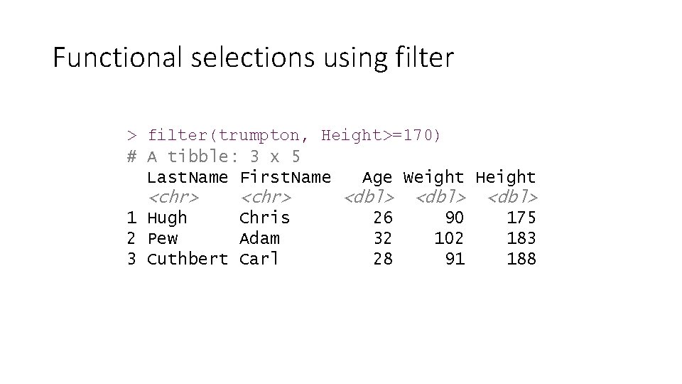
Functional selections using filter > filter(trumpton, Height>=170) # A tibble: 3 x 5 Last. Name First. Name Age Weight Height <chr> <dbl> 1 Hugh Chris 2 Pew Adam 3 Cuthbert Carl 26 32 28 90 102 91 175 183 188

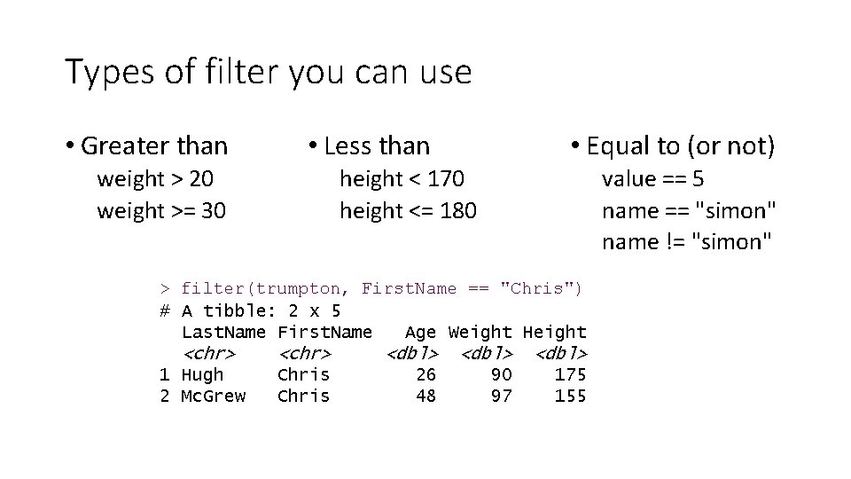
Types of filter you can use • Greater than • Less than • Equal to (or not) height < 170 height <= 180 weight > 20 weight >= 30 value == 5 name == "simon" name != "simon" > filter(trumpton, First. Name == "Chris") # A tibble: 2 x 5 Last. Name First. Name Age Weight Height <chr> 1 Hugh 2 Mc. Grew <chr> <dbl> Chris 26 48 90 97 175 155

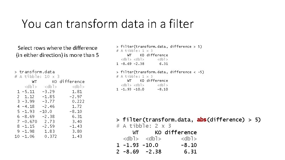
You can transform data in a filter Select rows where the difference (in either direction) is more than 5 > transform. data # A tibble: 10 x 3 WT KO difference <dbl> 1 -5. 11 -3. 29 1. 81 2 1. 12 -1. 85 -2. 97 3 -3. 99 -3. 77 0. 222 4 -4. 18 -2. 46 1. 72 5 -1. 93 -10. 0 -8. 10 6 -8. 69 -2. 38 6. 31 7 -0. 670 2. 73 3. 40 8 -1. 15 -2. 59 -1. 43 9 -1. 98 1. 83 3. 80 10 -1. 06 0. 372 1. 43 > filter(transform. data, difference > 5) # A tibble: 1 x 3 WT KO difference <dbl> 1 -8. 69 -2. 38 6. 31 > filter(transform. data, difference < -5) # A tibble: 1 x 3 WT KO difference <dbl> 1 -1. 93 -10. 0 -8. 10 > filter(transform. data, abs(difference) > 5) # A tibble: 2 x 3 WT KO difference <dbl> 1 -1. 93 -10. 0 -8. 10 2 -8. 69 -2. 38 6. 31

Exercise 4

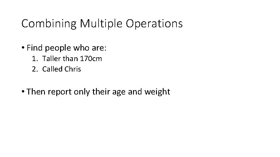
Combining Multiple Operations • Find people who are: 1. Taller than 170 cm 2. Called Chris • Then report only their age and weight

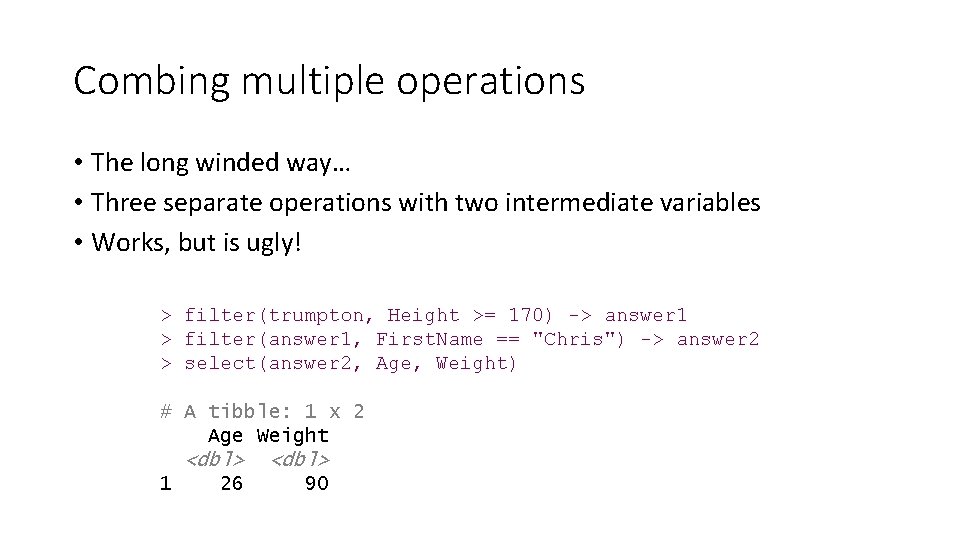
Combing multiple operations • The long winded way… • Three separate operations with two intermediate variables • Works, but is ugly! > filter(trumpton, Height >= 170) -> answer 1 > filter(answer 1, First. Name == "Chris") -> answer 2 > select(answer 2, Age, Weight) # A tibble: 1 x 2 Age Weight 1 <dbl> 26 90

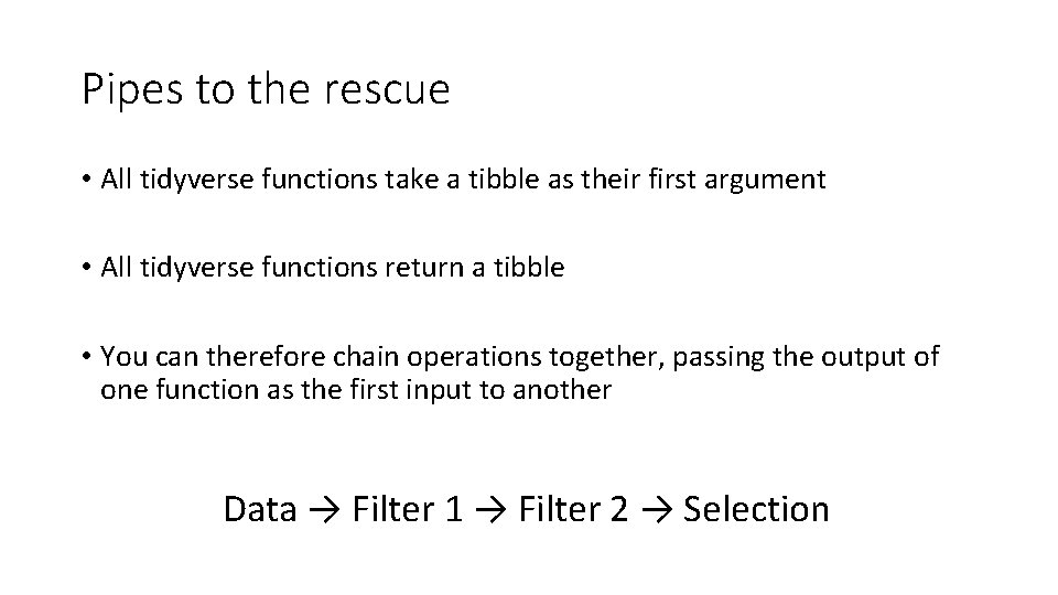
Pipes to the rescue • All tidyverse functions take a tibble as their first argument • All tidyverse functions return a tibble • You can therefore chain operations together, passing the output of one function as the first input to another Data → Filter 1 → Filter 2 → Selection

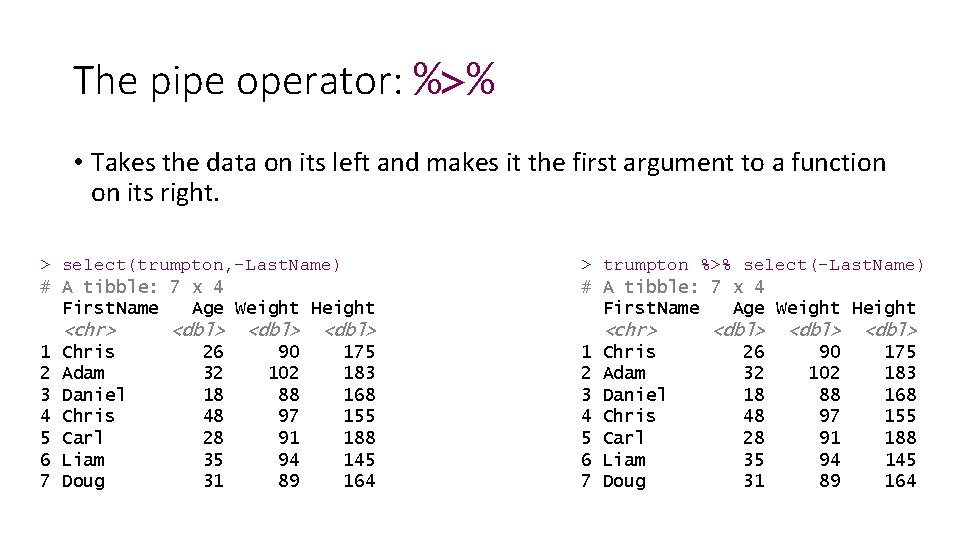
The pipe operator: %>% • Takes the data on its left and makes it the first argument to a function on its right. > select(trumpton, -Last. Name) # A tibble: 7 x 4 First. Name Age Weight Height <chr> 1 2 3 4 5 6 7 Chris Adam Daniel Chris Carl Liam Doug <dbl> 26 32 18 48 28 35 31 90 102 88 97 91 94 89 175 183 168 155 188 145 164 > trumpton %>% select(-Last. Name) # A tibble: 7 x 4 First. Name Age Weight Height <chr> 1 2 3 4 5 6 7 Chris Adam Daniel Chris Carl Liam Doug <dbl> 26 32 18 48 28 35 31 90 102 88 97 91 94 89 175 183 168 155 188 145 164

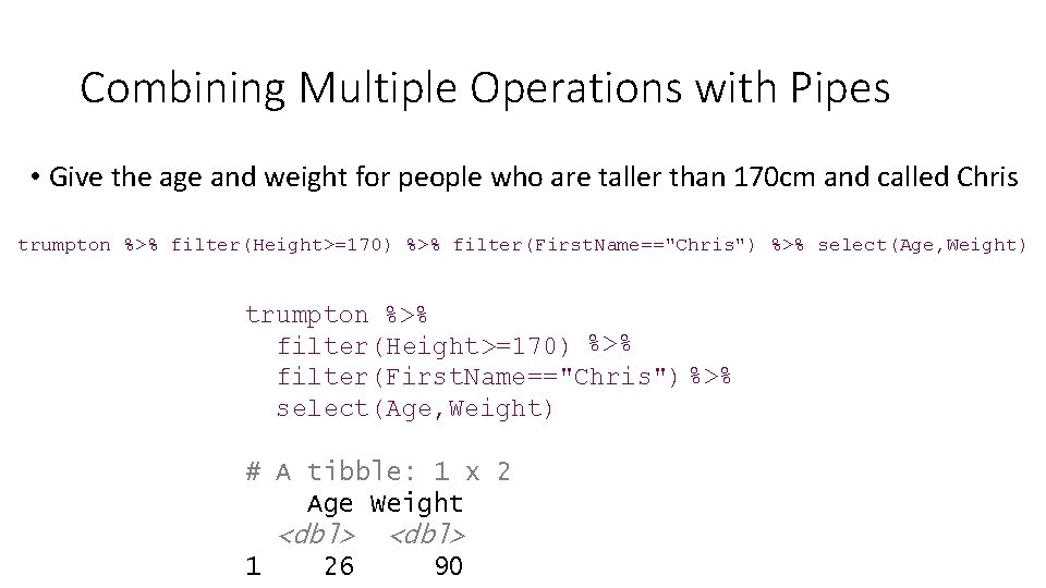
Combining Multiple Operations with Pipes • Give the age and weight for people who are taller than 170 cm and called Chris trumpton %>% filter(Height>=170) %>% filter(First. Name=="Chris") %>% select(Age, Weight) # A tibble: 1 x 2 Age Weight 1 <dbl> 26 90

Exercise 5

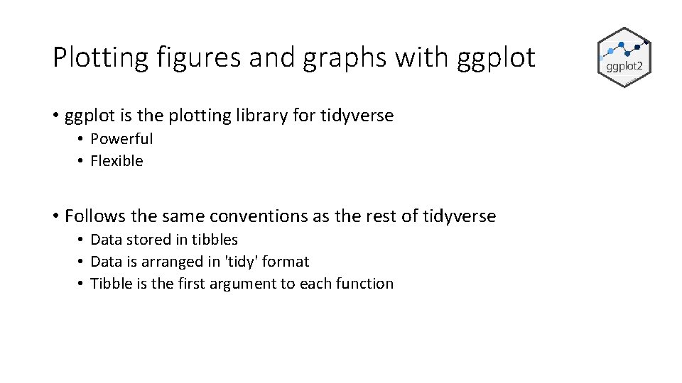
Plotting figures and graphs with ggplot • ggplot is the plotting library for tidyverse • Powerful • Flexible • Follows the same conventions as the rest of tidyverse • Data stored in tibbles • Data is arranged in 'tidy' format • Tibble is the first argument to each function

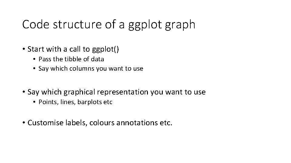
Code structure of a ggplot graph • Start with a call to ggplot() • Pass the tibble of data • Say which columns you want to use • Say which graphical representation you want to use • Points, lines, barplots etc • Customise labels, colours annotations etc.

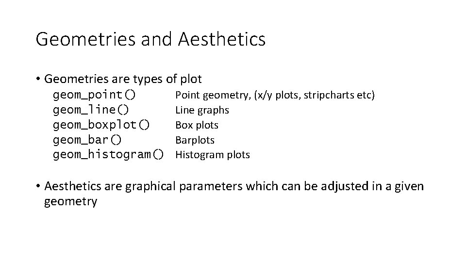
Geometries and Aesthetics • Geometries are types of plot geom_point() geom_line() geom_boxplot() geom_bar() geom_histogram() Point geometry, (x/y plots, stripcharts etc) Line graphs Box plots Barplots Histogram plots • Aesthetics are graphical parameters which can be adjusted in a given geometry

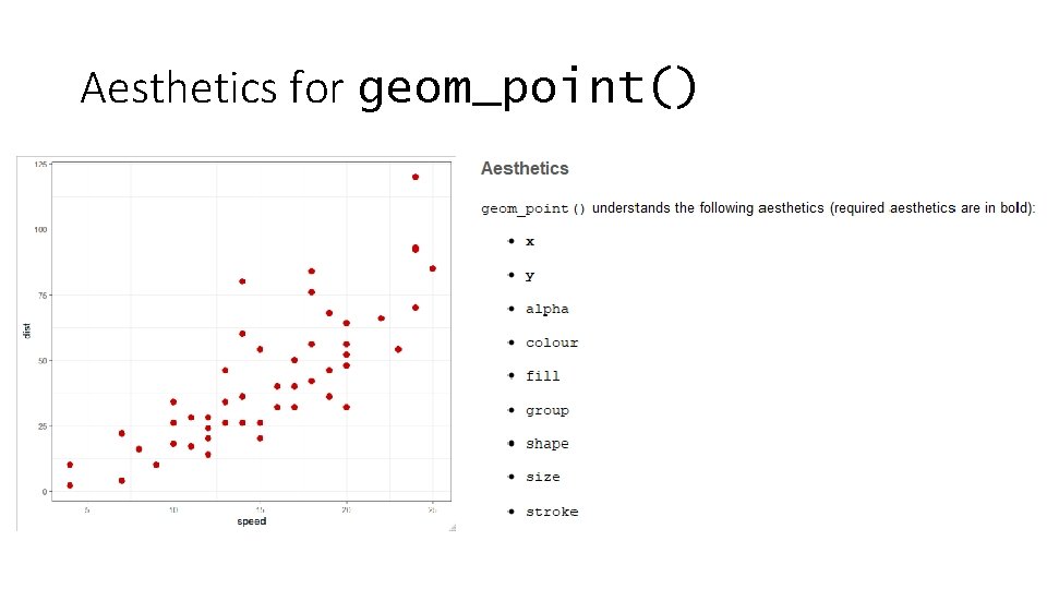
Aesthetics for geom_point()

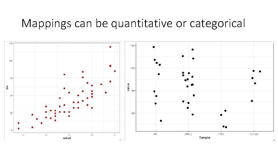
Mappings can be quantitative or categorical

How do you define aesthetics • Fixed values • Colour all points red • Make the points size 4 • Encoded from your data – called an aesthetic mapping • Colour according to genotype • Size based on the number of observations • Aesthetic mappings are set using the aes() function, normally as an argument to the ggplot function data %>% ggplot(aes(x=weight, y=height, colour=genotype))

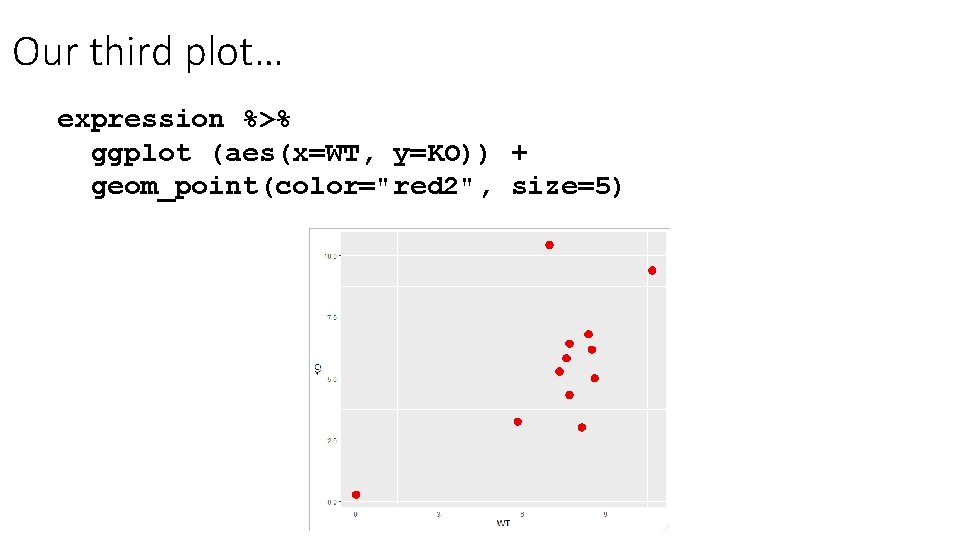
Putting things together • Identify the tibble with the data you want to plot • Decide on the geometry (plot type) you want to use • Decide which columns will modify which aesthetic • Call ggplot(aes(. . . )) • Add a geom_xxx function call

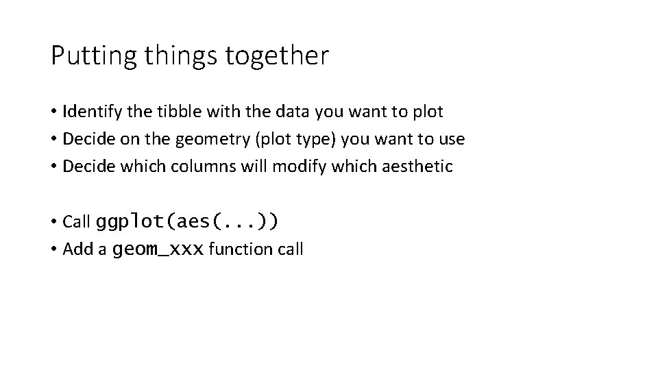
Our first plot… ggplot( expression, aes(x=WT, y=KO)) + geom_point() > expression # A tibble: 12 x 4 Gene WT KO p. Value <chr> <dbl> 1 Mia 1 5. 83 3. 24 0. 1 2 Snrpa 8. 59 5. 02 0. 001 3 Itpkc 8. 49 6. 16 0. 04 4 Adck 4 7. 69 6. 41 0. 2 5 Numbl 8. 37 6. 81 0. 1 6 Ltbp 4 6. 96 10. 4 0. 001 7 Shkbp 1 7. 57 5. 83 0. 1 8 Spnb 4 10. 7 9. 38 0. 2 9 Blvrb 7. 32 5. 29 0. 05 10 Pgam 1 0 0. 285 0. 5 11 Sertad 3 8. 13 3. 02 0. 0001 12 Sertad 1 7. 69 4. 34 0. 01 • Identify the tibble with the data you want to plot • Decide on the geometry (plot type) you want to use • Decide which columns will modify which aesthetic • Call ggplot(aes(. . . )) • Add a geom_xxx function call

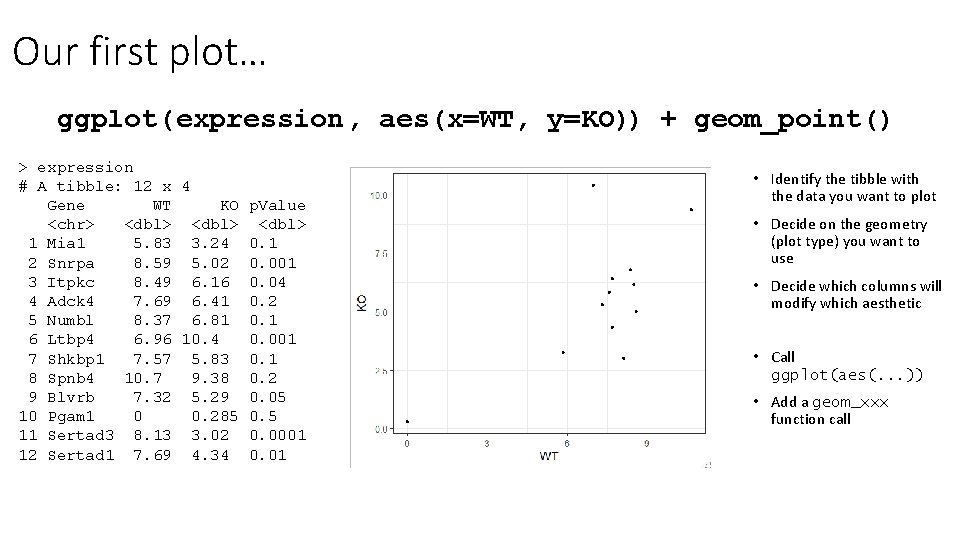
Our second plot… ggplot( expression, aes(x=WT, y=KO)) + geom_line() > expression # A tibble: 12 x 4 Gene WT KO p. Value <chr> <dbl> 1 Mia 1 5. 83 3. 24 0. 1 2 Snrpa 8. 59 5. 02 0. 001 3 Itpkc 8. 49 6. 16 0. 04 4 Adck 4 7. 69 6. 41 0. 2 5 Numbl 8. 37 6. 81 0. 1 6 Ltbp 4 6. 96 10. 4 0. 001 7 Shkbp 1 7. 57 5. 83 0. 1 8 Spnb 4 10. 7 9. 38 0. 2 9 Blvrb 7. 32 5. 29 0. 05 10 Pgam 1 0 0. 285 0. 5 11 Sertad 3 8. 13 3. 02 0. 0001 12 Sertad 1 7. 69 4. 34 0. 01

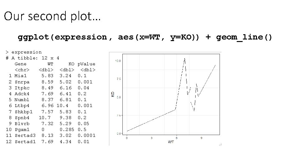
Our third plot… expression %>% ggplot (aes(x=WT, y=KO)) + geom_point(color="red 2", size=5)

Exercise 6

Other plot types • Barplots • geom_bar • geom_col • Histograms • geom_histogram • Density plots • geom_density

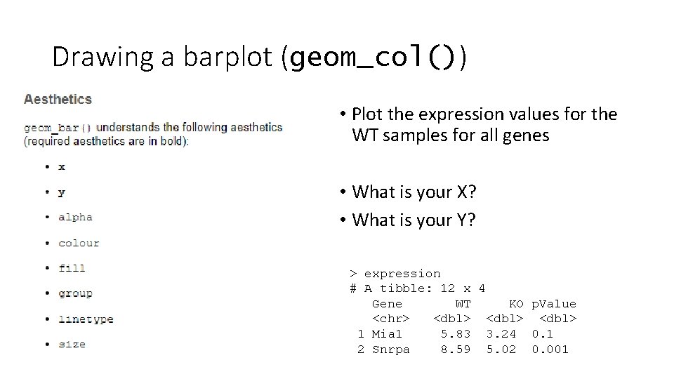
Drawing a barplot (geom_col()) • Plot the expression values for the WT samples for all genes • What is your X? • What is your Y? > expression # A tibble: 12 x 4 Gene WT KO p. Value <chr> <dbl> 1 Mia 1 5. 83 3. 24 0. 1 2 Snrpa 8. 59 5. 02 0. 001

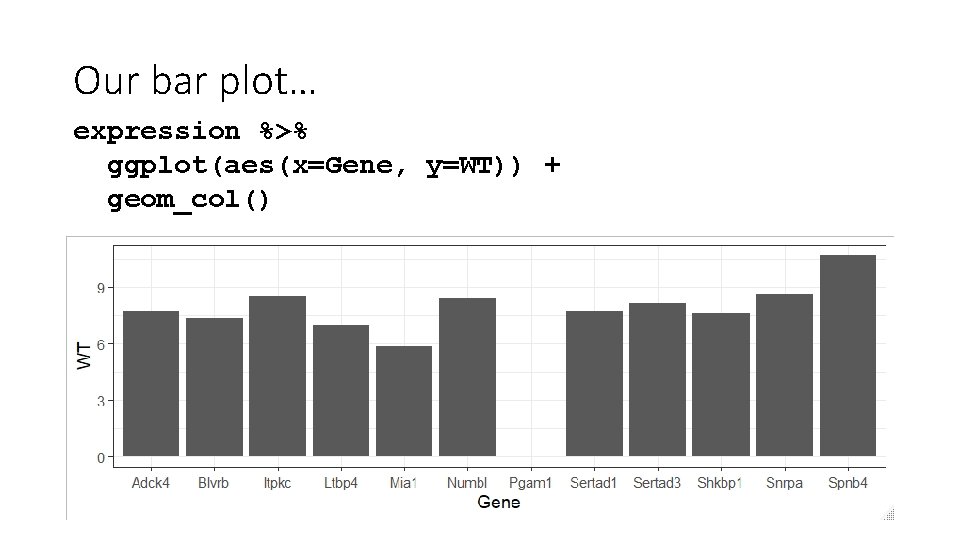
Our bar plot… expression %>% ggplot(aes(x=Gene, y=WT)) + geom_col()

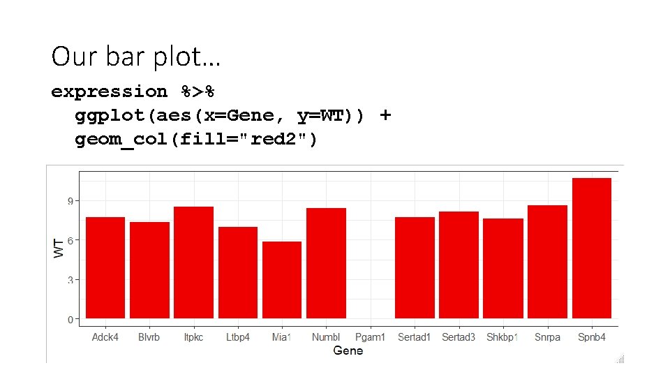
Our bar plot… expression %>% ggplot(aes(x=Gene, y=WT)) + geom_col(fill="red 2")

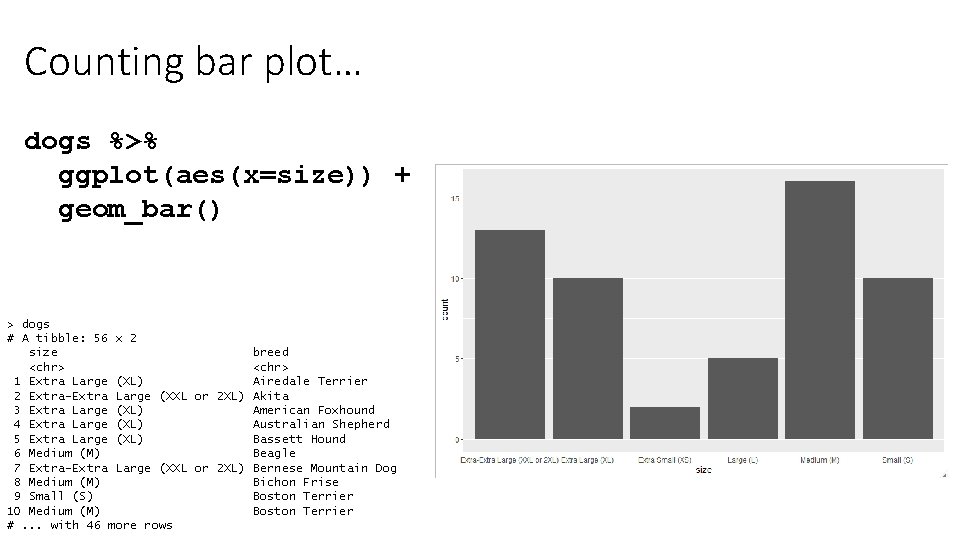
Counting bar plot… dogs %>% ggplot(aes(x=size)) + geom_bar() > dogs # A tibble: 56 x 2 size breed <chr> 1 Extra Large (XL) Airedale Terrier 2 Extra-Extra Large (XXL or 2 XL) Akita 3 Extra Large (XL) American Foxhound 4 Extra Large (XL) Australian Shepherd 5 Extra Large (XL) Bassett Hound 6 Medium (M) Beagle 7 Extra-Extra Large (XXL or 2 XL) Bernese Mountain Dog 8 Medium (M) Bichon Frise 9 Small (S) Boston Terrier 10 Medium (M) Boston Terrier #. . . with 46 more rows

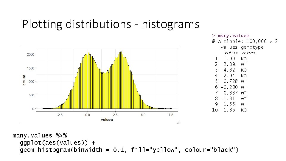
Plotting distributions - histograms > many. values # A tibble: 100, 000 x 2 values genotype <dbl> <chr> 1 1. 90 KO 2 2. 39 WT 3 4. 32 KO 4 2. 94 KO 5 0. 728 WT 6 -0. 280 WT 7 0. 337 WT 8 -1. 31 WT 9 1. 55 WT 10 1. 86 KO many. values %>% ggplot(aes(values)) + geom_histogram(binwidth = 0. 1, fill="yellow", colour="black")

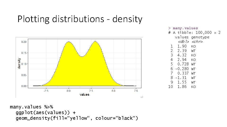
Plotting distributions - density > many. values # A tibble: 100, 000 x 2 values genotype <dbl> <chr> 1 1. 90 KO 2 2. 39 WT 3 4. 32 KO 4 2. 94 KO 5 0. 728 WT 6 -0. 280 WT 7 0. 337 WT 8 -1. 31 WT 9 1. 55 WT 10 1. 86 KO many. values %>% ggplot(aes(values)) + geom_density(fill="yellow", colour="black")

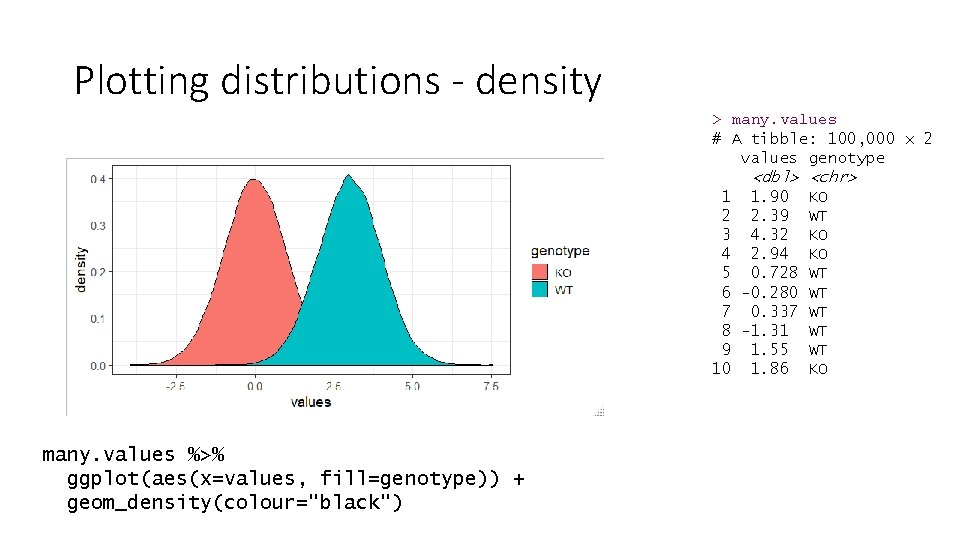
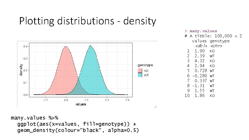
Plotting distributions - density > many. values # A tibble: 100, 000 x 2 values genotype <dbl> <chr> 1 1. 90 KO 2 2. 39 WT 3 4. 32 KO 4 2. 94 KO 5 0. 728 WT 6 -0. 280 WT 7 0. 337 WT 8 -1. 31 WT 9 1. 55 WT 10 1. 86 KO many. values %>% ggplot(aes(x=values, fill=genotype)) + geom_density(colour="black")

Plotting distributions - density > many. values # A tibble: 100, 000 x 2 values genotype <dbl> <chr> 1 1. 90 KO 2 2. 39 WT 3 4. 32 KO 4 2. 94 KO 5 0. 728 WT 6 -0. 280 WT 7 0. 337 WT 8 -1. 31 WT 9 1. 55 WT 10 1. 86 KO many. values %>% ggplot(aes(x=values, fill=genotype)) + geom_density(colour="black", alpha=0. 5)

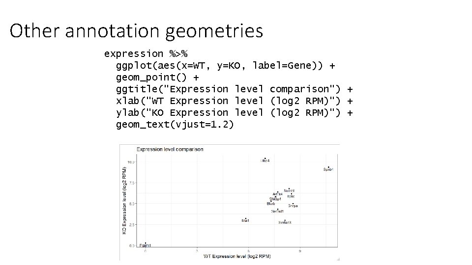
Other annotation geometries expression %>% ggplot(aes(x=WT, y=KO, label=Gene)) + geom_point() + ggtitle("Expression level comparison") + xlab("WT Expression level (log 2 RPM)") + ylab("KO Expression level (log 2 RPM)") + geom_text(vjust=1. 2)

Exercise 7