Introduction to R Basics Based on R tutorial

Introduction to R Basics * Based on R tutorial by Lorenza Bordoli

R-project background • Origin and History – initially written by Ross Ihaka and Robert Gentleman at Dep. of Statistics of U of Auckland, New Zealand during 1990 s. – International project since 1997 • Open source with GPL license – Free to anyone – In actively development – http: //www. r-project. org/

What R does R is a programming environment for statistical and data analysis computations. • Core Package • Statistical functions • plotting and graphics • Data handling and storage • predefined data reader • textual, regular expressions • hashing • Data analysis functions • Programming support: • loops, branching, subroutines • Object Oriented • More additional developed packages.

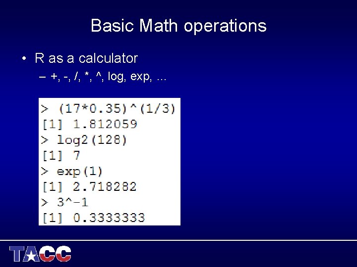
Basic Math operations • R as a calculator – +, -, /, *, ^, log, exp, …

Variables • Numeric • Character String • Logical

Assigning Values to Variables • “<-” or “=“ • Assign multiple values – Concatenate, c() – From stdin, scan() – Series • : • Seq()

NA: Missing Value • Variables of each data type (numeric, character, logical) can also take the value NA: not available. • NA is not the same as 0 • NA is not the same as “” • NA is not the same as FALSE • Any operations (calculations, comparisons) that involve NA may or may not produce NA:

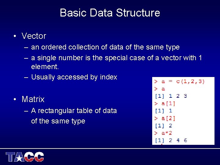
Basic Data Structure • Vector – an ordered collection of data of the same type – a single number is the special case of a vector with 1 element. – Usually accessed by index • Matrix – A rectangular table of data of the same type

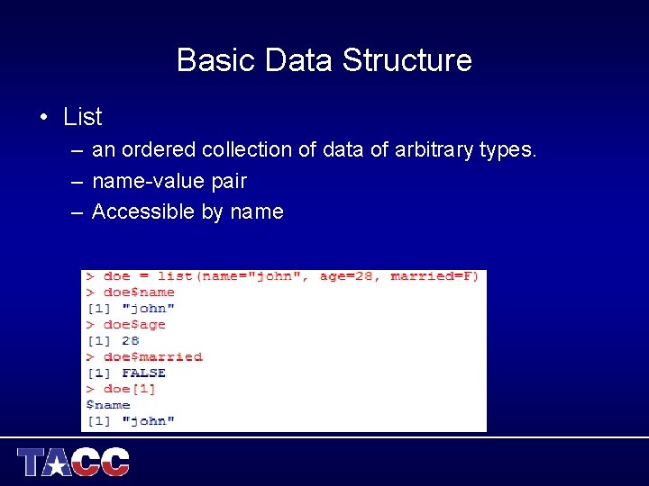
Basic Data Structure • List – an ordered collection of data of arbitrary types. – name-value pair – Accessible by name

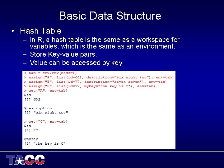
Basic Data Structure • Hash Table – In R, a hash table is the same as a workspace for variables, which is the same as an environment. – Store Key-value pairs. – Value can be accessed by key

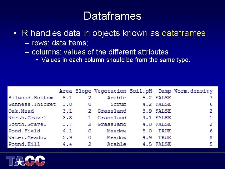
Dataframes • R handles data in objects known as dataframes; – rows: data items; – columns: values of the different attributes • Values in each column should be from the same type.

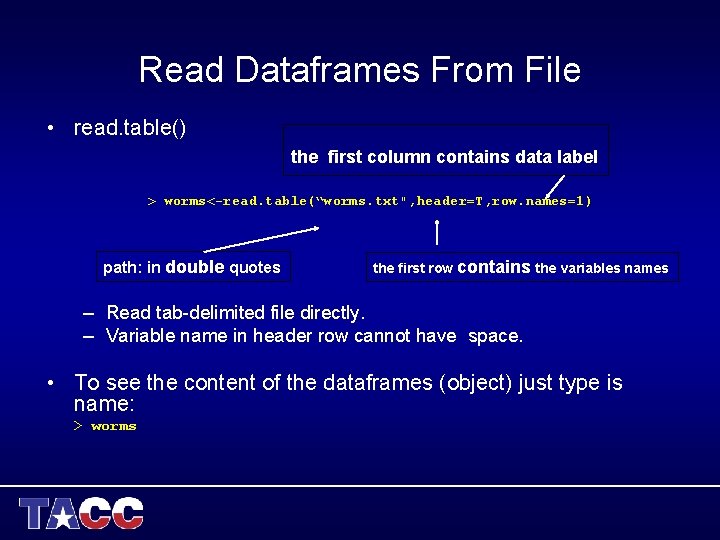
Read Dataframes From File • read. table() the first column contains data label > worms<-read. table(“worms. txt", header=T, row. names=1) path: in double quotes the first row contains the variables names – Read tab-delimited file directly. – Variable name in header row cannot have space. • To see the content of the dataframes (object) just type is name: > worms

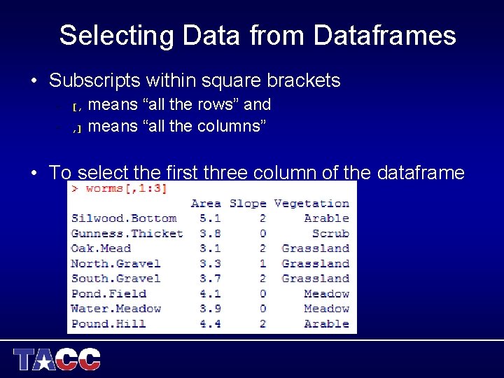
Selecting Data from Dataframes • Subscripts within square brackets means “all the rows” and , ] means “all the columns” – [, – • To select the first three column of the dataframe

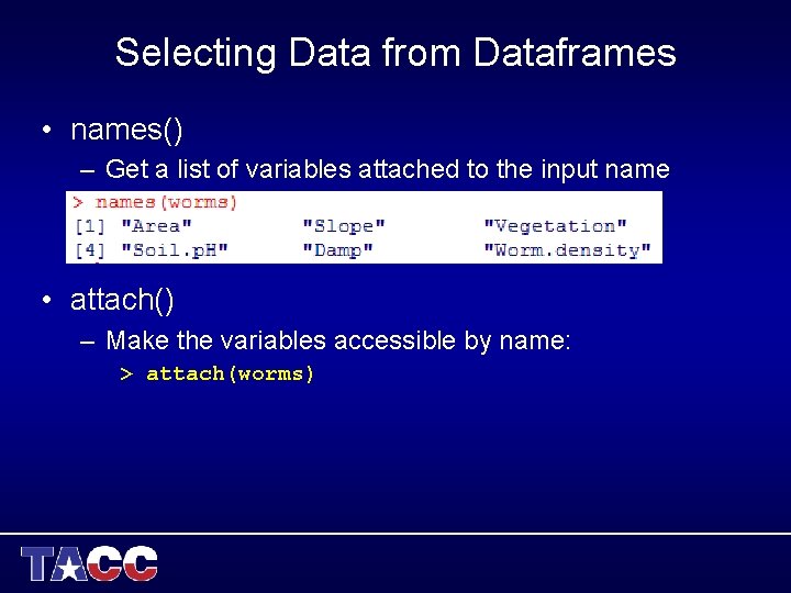
Selecting Data from Dataframes • names() – Get a list of variables attached to the input name • attach() – Make the variables accessible by name: > attach(worms)

Selecting Data from Dataframes • Using logic expression while selecting:

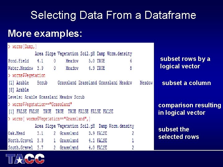
Selecting Data From a Dataframe More examples: subset rows by a logical vector subset a column comparison resulting in logical vector subset the selected rows

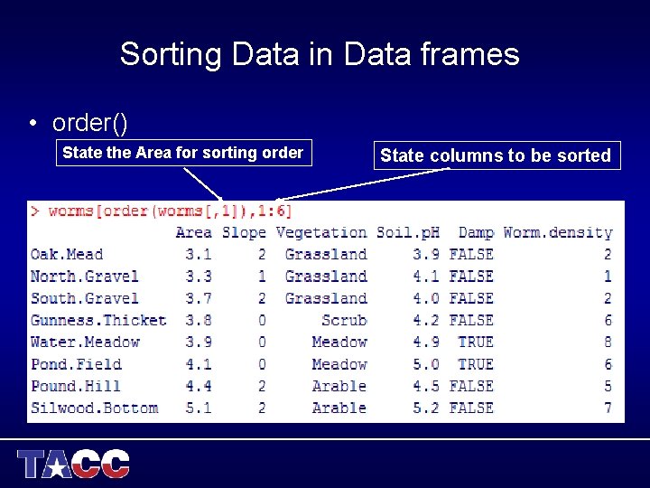
Sorting Data in Data frames • order() State the Area for sorting order State columns to be sorted >worms[order(worms[, 1]), 1: 6] Area Slope Vegetation Soil. p. H Damp Worm. density Farm. Wood 0. 8 10 Scrub 5. 1 TRUE Rookery. Slope 1. 5 4 Grassland 5. 0 TRUE Observatory. Ridge 1. 8 6 Grassland 3. 8 FALSE The. Orchard 1. 9 0 Orchard 5. 7 FALSE Ashurst 2. 1 0 Arable 4. 8 FALSE Cheapside 2. 2 8 Scrub 4. 7 TRUE Rush. Meadow 2. 4 5 Meadow 4. 9 TRUE Nursery. Field 2. 8 3 Grassland 4. 3 FALSE (…) 3 7 0 9 4 4 5 2

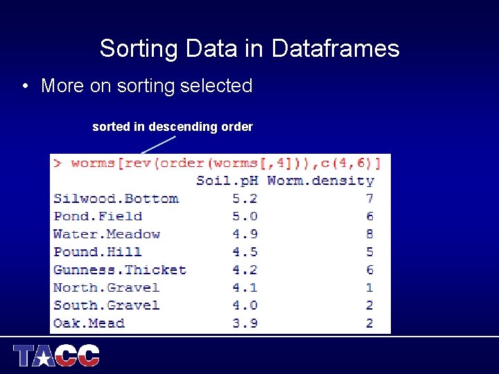
Sorting Data in Dataframes • More on sorting selected sorted in descending order

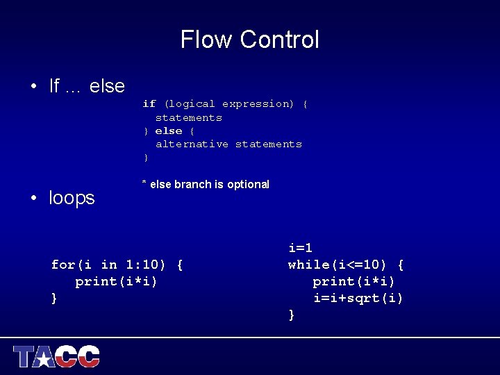
Flow Control • If … else if (logical expression) { statements } else { alternative statements } • loops * else branch is optional for(i in 1: 10) { print(i*i) } i=1 while(i<=10) { print(i*i) i=i+sqrt(i) }

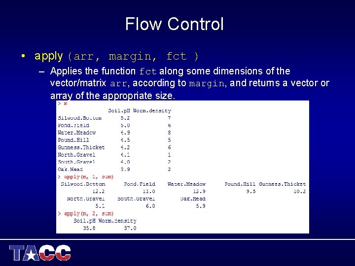
Flow Control • apply (arr, margin, fct ) – Applies the function fct along some dimensions of the vector/matrix arr, according to margin, and returns a vector or array of the appropriate size.

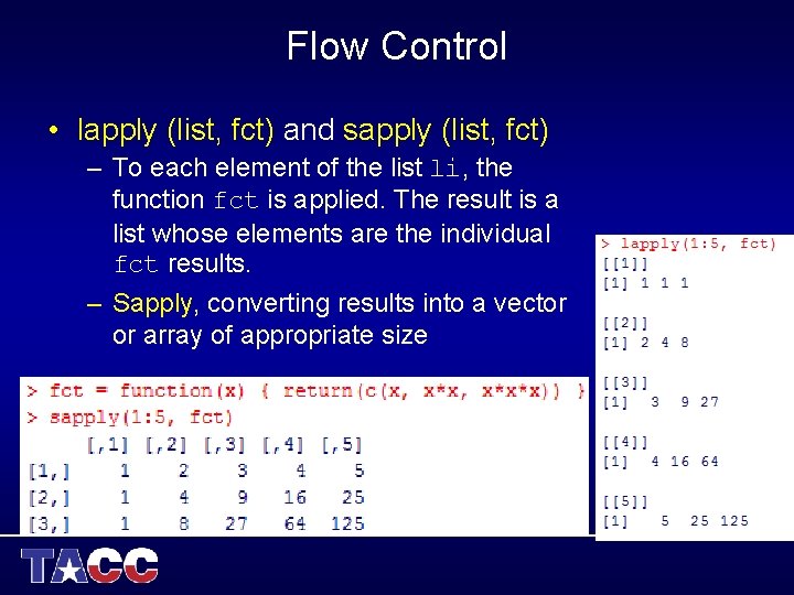
Flow Control • lapply (list, fct) and sapply (list, fct) – To each element of the list li, the function fct is applied. The result is a list whose elements are the individual fct results. – Sapply, converting results into a vector or array of appropriate size

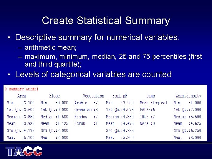
Create Statistical Summary • Descriptive summary for numerical variables: – arithmetic mean; – maximum, minimum, median, 25 and 75 percentiles (first and third quartile); • Levels of categorical variables are counted

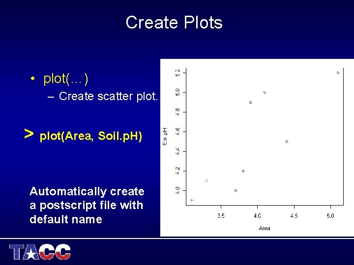
Create Plots • plot(…) – Create scatter plot. > plot(Area, Soil. p. H) Automatically create a postscript file with default name

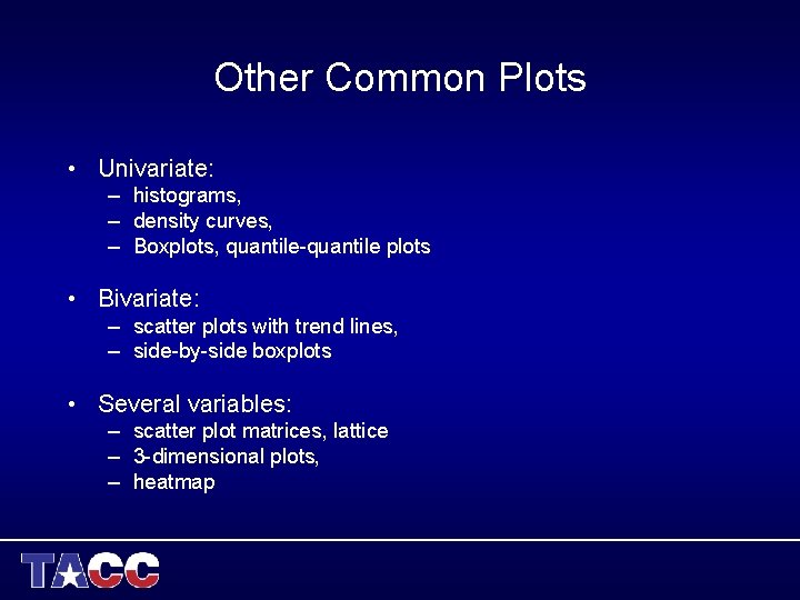
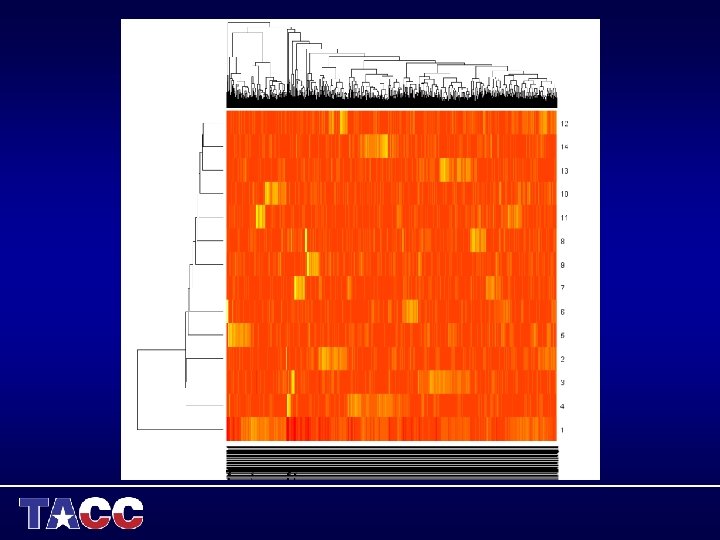
Other Common Plots • Univariate: – histograms, – density curves, – Boxplots, quantile-quantile plots • Bivariate: – scatter plots with trend lines, – side-by-side boxplots • Several variables: – scatter plot matrices, lattice – 3 -dimensional plots, – heatmap

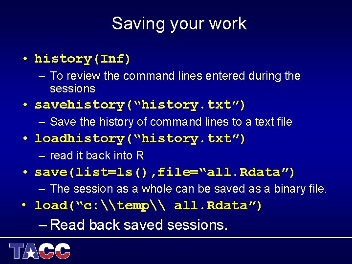
Saving your work • history(Inf) – To review the command lines entered during the sessions • savehistory(“history. txt”) – Save the history of command lines to a text file • loadhistory(“history. txt”) – read it back into R • save(list=ls(), file=“all. Rdata”) – The session as a whole can be saved as a binary file. • load(“c: \temp\ all. Rdata”) – Read back saved sessions.

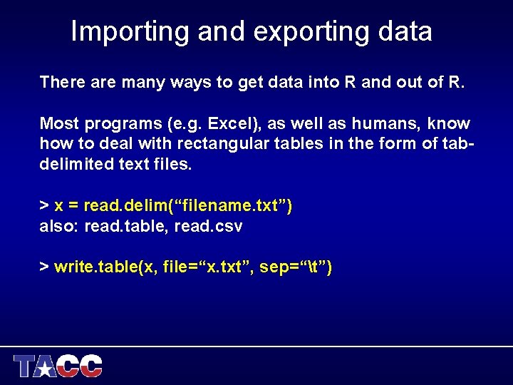
Importing and exporting data There are many ways to get data into R and out of R. Most programs (e. g. Excel), as well as humans, know how to deal with rectangular tables in the form of tabdelimited text files. > x = read. delim(“filename. txt”) also: read. table, read. csv > write. table(x, file=“x. txt”, sep=“t”)

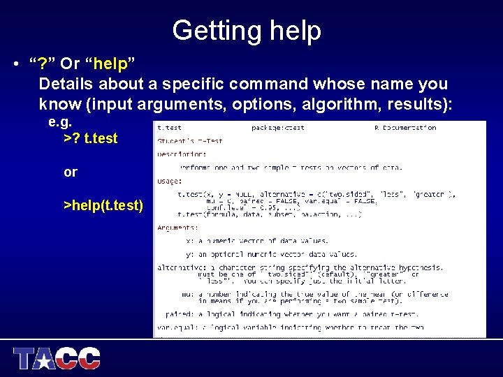
Getting help • “? ” Or “help” Details about a specific command whose name you know (input arguments, options, algorithm, results): e. g. >? t. test or >help(t. test)

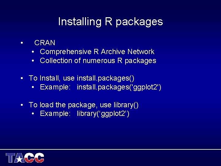
Installing R packages • CRAN • Comprehensive R Archive Network • Collection of numerous R packages • To Install, use install. packages() • Example: install. packages('ggplot 2') • To load the package, use library() • Example: library(‘ggplot 2’)

Data Mining with R

Data mining with R • Many data mining methods are also supported in R core package or in R modules – Kmeans clustering: • Kmeans() – Decision tree: • rpart() in rpart library – Nearest Neighbour • Knn() in class library –…

Additional Libraries and Packages • Libraries – Comes with Package installation (Core or others) – library() shows a list of current installed – library must be loaded before use e. g. • library(rpart) • Packages – Developed code/libraries outside the core packages – Can be downloaded and installed separately • Install. package(“name”) – There are currently 2561 packages at http: //cran. rproject. org/web/packages/ • E. g. Rweka, interface to Weka.

Common Data Mining Methods • Clustering analysis – Grouping data object into different bucket. – Common methods: • Distance based clustering, e. g. k-means • Density based clustering e. g. DBSCAN • Hierarchical clustering e. g. Aggregative hierarchical clustering • Classification – Assigning labels to each data object based on training data. – Common methods: • Distance based classification: e. g. SVM • Statistic based classification: e. g. Naïve Bayesian • Rule based classification: e. g. Decision tree classification

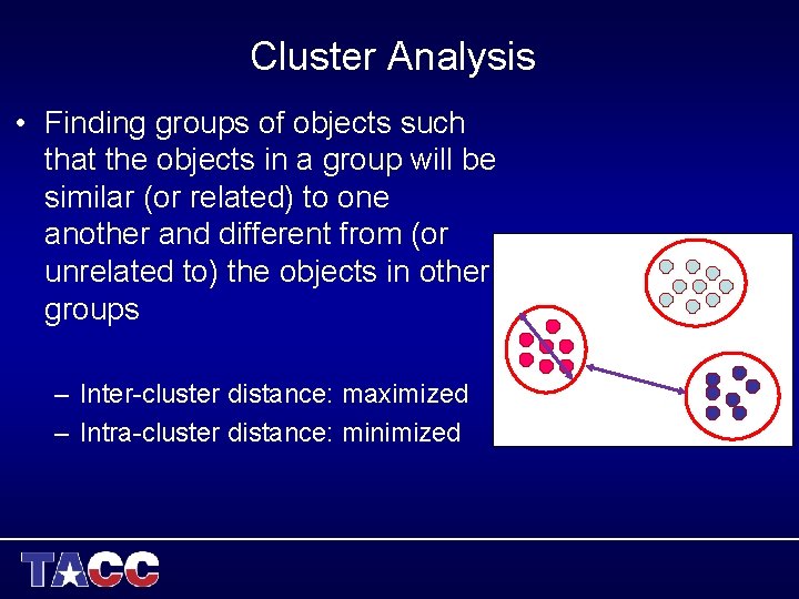
Cluster Analysis • Finding groups of objects such that the objects in a group will be similar (or related) to one another and different from (or unrelated to) the objects in other groups – Inter-cluster distance: maximized – Intra-cluster distance: minimized

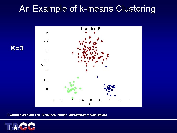
An Example of k-means Clustering K=3 Examples are from Tan, Steinbach, Kumar Introduction to Data Mining

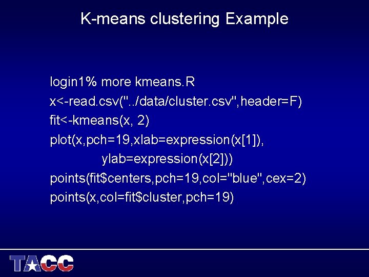
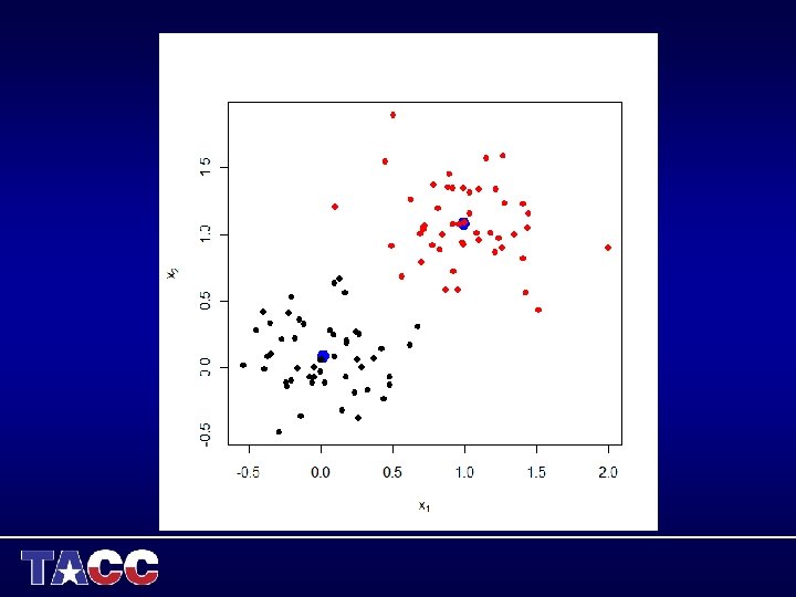
K-means clustering Example login 1% more kmeans. R x<-read. csv(". . /data/cluster. csv", header=F) fit<-kmeans(x, 2) plot(x, pch=19, xlab=expression(x[1]), ylab=expression(x[2])) points(fit$centers, pch=19, col="blue", cex=2) points(x, col=fit$cluster, pch=19)

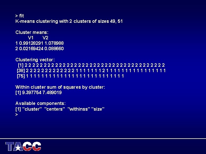
> fit K-means clustering with 2 clusters of sizes 49, 51 Cluster means: V 1 V 2 1 0. 99128291 1. 078988 2 0. 02169424 0. 088660 Clustering vector: [1] 2 2 2 2 2 2 2 2 2 2 [38] 2 2 2 2 1 1 1 1 1 1 [75] 1 1 1 1 1 1 1 Within cluster sum of squares by cluster: [1] 9. 397754 7. 489019 Available components: [1] "cluster" "centers" "withinss" "size" >

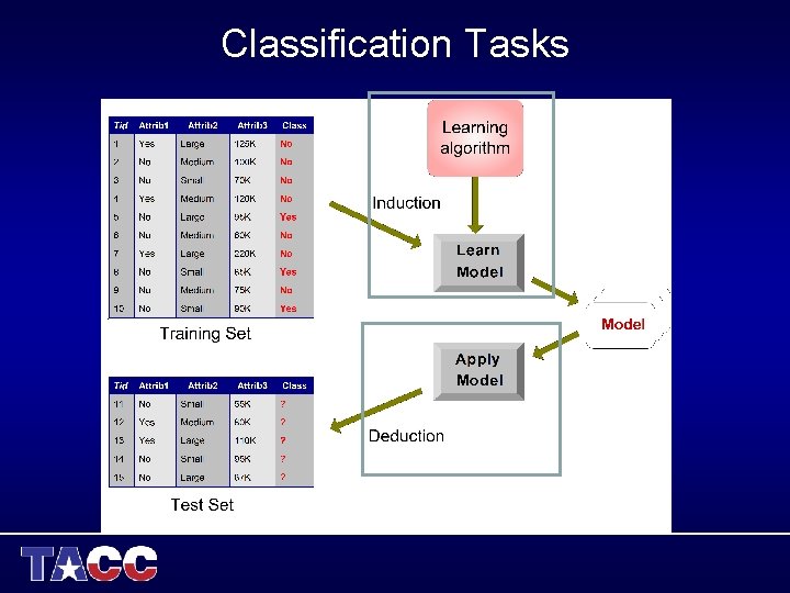
Classification Tasks

Support Vector Machine Classification • A distance based classification method. • The core idea is to find the best hyperplane to separate data from two classes. • The class of a new object can be determined based on its distance from the hyperplane.

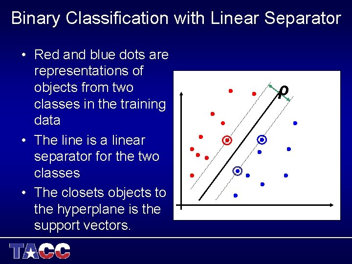
Binary Classification with Linear Separator • Red and blue dots are representations of objects from two classes in the training data • The line is a linear separator for the two classes • The closets objects to the hyperplane is the support vectors. ρ

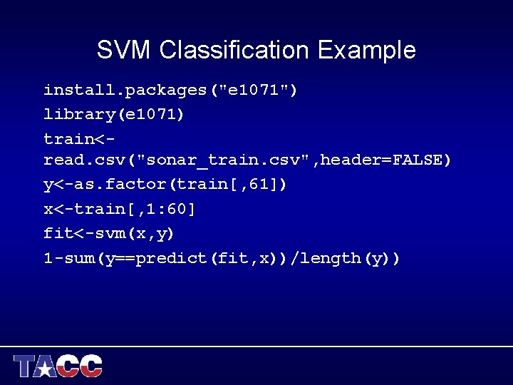
SVM Classification Example install. packages("e 1071") library(e 1071) train<read. csv("sonar_train. csv", header=FALSE) y<-as. factor(train[, 61]) x<-train[, 1: 60] fit<-svm(x, y) 1 -sum(y==predict(fit, x))/length(y))

SVM Classification Example test<read. csv("sonar_test. csv", header=FALSE) y_test<-as. factor(test[, 61]) x_test<-test[, 1: 60] 1 sum(y_test==predict(fit, x_test))/length (y_test)

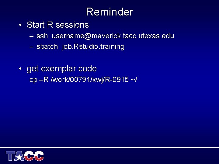
Reminder • Start R sessions – ssh username@maverick. tacc. utexas. edu – sbatch job. Rstudio. training • get exemplar code cp –R /work/00791/xwj/R-0915 ~/

Further references • R – M. Crawley, Statistics An Introduction using R, Wiley – J. Verzani, Simple. R Using R for Introductory Statistics http: //cran. r-project. org/doc/contrib/Verzani-Simple. R. pdf – Programming manual: • http: //cran. r-project. org/manuals. html • Using R for data mining – Data Mining with R: Learning with case studies, Luis Togo • Contact Info – Weijia Xu xwj@tacc. utexas. edu

End of Morning Session • Get on the Maverick and start R sessions • Basics of R – Variable types – Data structure – Flow controls • Using R for data mining – Code examples.

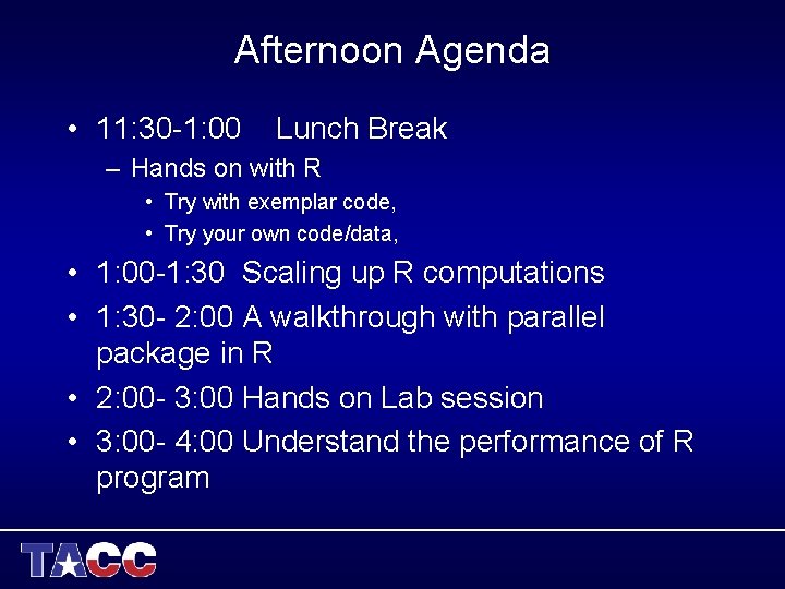
Afternoon Agenda • 11: 30 -1: 00 Lunch Break – Hands on with R • Try with exemplar code, • Try your own code/data, • 1: 00 -1: 30 Scaling up R computations • 1: 30 - 2: 00 A walkthrough with parallel package in R • 2: 00 - 3: 00 Hands on Lab session • 3: 00 - 4: 00 Understand the performance of R program