Introduction to R and R Studio Consider A

Introduction to R and R Studio

� Consider ◦ ◦ �A the tasks you will need to perform Data collection and editing? Data transformation/calculations? Basic vs. advanced statistics? Making figures? single platform may not be enough, but use as few as possible Software Mac PC Data entry/ Forms Data editing Transform data Basic stats Adv statics Figures REDCap web +++ - - - + X ++ ++ ++ X X ++ ++ R/RStudio X X - + +++ +++ Epi Info Open Office

Agenda � About R and R Studio � Why and when do I use R? � Key Features � How does it fit in with other tools? � Basic tasks � Example – Import and analyze the Framingham dataset

About R and R Studio � Open source statistical analysis software � Large development community ◦ Many translational analysis packages only in R ◦ Lots of on-line help and examples � https: //www. r-project. org (R basic) ◦ EVERYTHING requires typed in commands � https: //www. rstudio. com ◦ ◦ (R + GUI wrapper) Easier to load and inspect files Assorted convenient extensions Still a lot of typed commands Suggest starting with R Studio

Why and when should I use R? � For any data manipulation for analysis beyond what Epi Info and Calc/Excel can do ◦ ◦ Complex regression and survival analysis Clustering analysis (all kinds) Times series analysis Translational and ‘omic’ analysis � Control of appearance of analysis output � When you need to make complex or high quality figures ◦ Heat maps ◦ Multiple panes, axes, colors ◦ Forest-type and other specialized plot types

Key features of R � ‘Command-line’ software � Can store and analyze very large datasets (100 s of millions of rows) � Extremely flexible in almost all commands ◦ Includes plot functions � Has analysis packages not available for anything else (vs. SAS, Stata, SPSS) ◦ Bioconductor!! � Many public data repositories include R commands to access and analyse (e. g. GEO) � Can automate analysis (e. g. generate many results form a single set of commands)

Rstudio - features

Excel vs. R Studio

Heat maps

Forest plots

How does R fit in with other tools? � Can connect to SQL servers and run commands � Can do complex power calculations � Usually the FINAL step in analysis pipeline ◦ After data collected and organized � Can be used for QC, (esp. large datasets) � Most robust statistical results � Generates final tables, results, and figures for interpretation and publication from data created elsewhere

Why not use R all the time? � Cannot use for data entry � Data manipulation is less intuitive ◦ Need some understanding of matrix manipulation � Harder to share results with others (e. g. like emailing an Excel file) � Takes some time to get comfortable with the commands ◦ Slower than Excel/Calc for some simple tasks like viewing results or simple sorting

Summary �R is a powerful analysis package that can perform statistics, make figures, and manipulate data � R is controlled using statements with a specific format less intuitive than other tools � R CANNOT be used as a database or to collect data

Resources for R � Content § § Reading http: //www. cyclismo. org/tutorial/R Bioinformatics Tzubioinformatics http: // compbio. ucdenver. edu/Hunter_lab/Phang/. . . /Bioinformatics/bioinformatics. html � Practice § § § by Doing http: //tryr. codeschool. com/ http: //www. statmethods. net/ http: //swirlstats. com/

Practical R overview

R statistical package

R Studio Datasets Data points Plots Commands

R packages �R has a lot of built-in functions � HOWEVER, real power is in ‘packages’ �devtools/tmap package

Spatial analysis � Population maps � Disease incidence � Environmental variables

Loading packages into R 1. Download package using window browser

Loading packages into R � Using command line: ◦ install. packages("xlsx") � Packages often use other packages ◦ You may need ”install dependencies”, or other packages that your package needs

Load library for use � Once you have installed a package, you must tell R to use it: � Window version (R Studio): � Command line: library(“xlsx”)

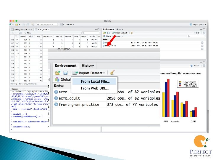
Loading data into R Studio 1. Command line – use ‘read’ command ◦ mydata <- read. csv(‘~/Desktop/mydata. csv’) ◦ myxlsx <- read. xlsx(‘~/Desktop/mydata. xslx’) �Must load ‘library(xlsx)’ 2. ◦ 3. ◦ R Studio GUI ‘Environment’ -> ‘Import dataset’ -> navigate to file > ‘Open’ Creates a data ‘frame’ containing file data Can have many components of different types � E. g. number, string, factor, Simplest is a table where columns are called by names ◦ � � fram$id = a list of all ids in the fram table Column sexc of fram where randid: fram$MF 4[fram$randid==2448]

Inspecting your data � To see column names, use names() ◦ E. g. names(fram) � To see all data in a “frame”, type its name � To see a specific column, use $ ◦ fram$sex � To see a few rows, treat it as a matrix ◦ 1 st 10 rows: fram[1: 10, ] � To see just a few columns, can use numbers or names: ◦ fram[, 1: 5] ◦ fram[, c(‘randid’, sex’, ’diabetes’, ’prevmi’, ’bmi’)

Making a simple summary table � Simple counts: ◦ Single variable: table(fram$sex); table(fram$educ) ◦ Two variables: table(fram$educ, fram$sex)

Make a more complex table � Use library gmodels ◦ library(gmodels) � Cross. Table function ◦ Cross. Table(fram$MF 79, fram$MF 71) � Remove proportion of total subjects ◦ Cross. Table(fram$MF 79, fram$MF 71, prop. t=FALSE) � Remove chi-squared contribution and proportion of column ◦ Cross. Table(fram$MF 79, fram$MF 71, prop. t=FALSE, prop. chisq=FALSE, prop. c=FALSE) � Add chi-square test ◦ Cross. Table(fram$MF 79, fram$MF 71, prop. t=FALSE, prop. chisq=FALSE, prop. c=FALSE, chisq=TRUE))

Make a more complex table � Use library gmodels ◦ library(gmodels) � Cross. Table function ◦ Cross. Table(fram$educ, fram$sex) � Remove proportion of total subjects ◦ Cross. Table(fram$educ, fram$sex, prop. t=FALSE) � Remove chi-squared contribution and proportion of column ◦ Cross. Table(fram$educ, fram$sex, prop. t=FALSE, prop. chisq=FALSE, prop. c=FALSE) � Add chi-square test ◦ Cross. Table(fram$educ, fram$sex, prop. t=FALSE, prop. chisq=FALSE, prop. c=FALSE, chisq=TRUE)

Make a simple plot � Basic plot function ◦ plot(fram$bmi, fram$sysbp) � Add chart labels ◦ plot(fram$bmi, fram$sysbp, xlab='BMI, kg/m 2', ylab='SBP, mm Hg', main='BMI vs. SBP')Change the appearance of the points ◦ plot(fram$bmi, fram$sysbp, xlab='BMI, kg/m 2', ylab='SBP, mm Hg', main='BMI vs. SBP', pch=17. col=‘blue’)

Make a simple plot � Basic plot function ◦ plot(fram$bmi, fram$sysbp) � Add chart labels ◦ plot(fram$bmi, fram$sysbp, xlab='BMI, kg/m 2', ylab='SBP, mm Hg', main='BMI vs. SBP')Change the appearance of the points ◦ plot(fram$bmi, fram$sysbp, xlab='BMI, kg/m 2', ylab='SBP, mm Hg', main='BMI vs. SBP', pch=17. col=‘blue’)

Regression example �R uses ’formula’ statements ◦ Dependent_var~var. A+var. B+var. C… � Linear regression ◦ Dependent variable is continuous (e. g. weight, BP) ◦ bmi~sex+educ ◦ Summary(glm(bmi~as. factor(sex)+educ, data=fram, family=gaussian)) � Logistic regression ◦ Dependent variable is dichotomous (Yes/No) ◦ anychd~sex+educ+bmi ◦ glm(anychd~as. factor(sex)+as. factor(educ)+ bmi, data=fram, family=binomial(link=“logit”))

Regression example �R uses ’formula’ statements ◦ Dependent_var~var. A+var. B+var. C… � Linear regression ◦ Dependent variable is continuous (e. g. weight, BP) ◦ bmi~sex+educ ◦ Summary(glm(bmi~as. factor(sex)+educ, data=fram, family=gaussian)) � Logistic regression ◦ Dependent variable is dichotomous (Yes/No) ◦ anychd~sex+educ+bmi ◦ glm(anychd~as. factor(sex)+as. factor(educ)+ bmi, data=fram, family=binomial(link=“logit”))

Practice � Make a table of educ vs. diabetes � Make a plot of age vs. sysbp � Perform a linear regression of systolic blood pressure sysbp vs. cursmoke, sex, and age � Perform a logistic regression of death vs. sex, diabetes, and cursmoke