Introduction to Queueing Theory Motivation v First developed

Introduction to Queueing Theory

Motivation v. First developed to analyze statistical behavior of phone switches.

Queueing Systems vmodel processes in which customers arrive. vwait their turn for service. v are serviced and then leave.

Examples vsupermarket checkouts stands. v world series ticket booths. v doctors waiting rooms etc. .

Five components of a Queueing system: v 1. Interarrival-time probability density function (pdf) v 2. service-time pdf v 3. Number of servers v 4. queueing discipline v 5. size of queue.

ASSUME van infinite number of customers (i. e. long queue does not reduce customer number).

Assumption is bad in : va time-sharing model. vwith finite number of customers. vif half wait for response, input rate will be reduced.

Interarrival-time pdf vrecord elapsed time since previous arrival. vlist the histogram of interarrival times (i. e. 10 0. 1 sec, 20 0. 2 sec. . . ). v. This is a pdf character.

Service time vhow long in the server? vi. e. one customer has a shopping cart full the other a box of cookies. v. Need a PDF to analyze this.

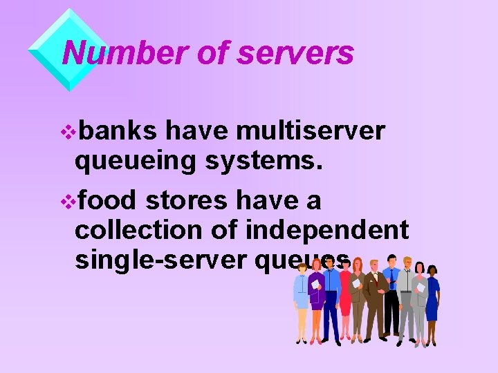
Number of servers vbanks have multiserver queueing systems. vfood stores have a collection of independent single-server queues.

Queueing discipline vorder of customer process -ing. v i. e. supermarkets are firstcome-first served. v. Hospital emergency rooms use sickest first.

Finite Length Queues v. Some queues have finite length: when full customers are rejected.

ASSUME vinfinite-buffer. vsingle-server system with first-come. v first-served queues.

A/B/m notation v. A=interarrival-time v. B=service-time pdf vm=number of servers.

A, B are chosen from the set: v. M=exponential pdf (M stands for Markov) v. D= all customers have the same value (D is for deterministic) v. G=general (i. e. arbitrary pdf)

Analysibility v. M/M/1 is known. v. G/G/m is not.

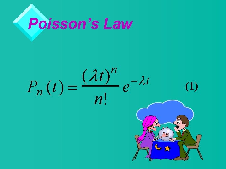
M/M/1 system v. For M/M/1 the probability of exactly n customers arriving during an interval of length t is given by the Poisson law.

Poisson’s Law n ( l t) - l t Pn (t ) = e n! (1)

Poisson’s Law in Physics vradio active decay –P[k alpha particles in t seconds] – = avg # of prtcls per second

Poisson’s Law in Operations Research vplanning sizes switchboard –P[k calls in t seconds] – =avg number of calls per sec

Poisson’s Law in Biology vwater pollution monitoring –P[k coliform bacteria in 1000 CCs] – =avg # of coliform bacteria per cc

Poisson’s Law in Transportation vplanning size of highway tolls –P[k autos in t minutes] – =avg# of autos per minute

Poisson’s Law in Optics vin designing an optical recvr –P[k photons per sec over the surface of area A] – =avg# of photons per

Poisson’s Law in Communications in designing a fiber optic xmit-rcvr link v –P[k photoelectrons generated at the rcvr in one second] – =avg # of photoelectrons per sec.

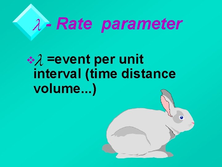
l - Rate parameter l =event per unit v interval (time distance volume. . . )

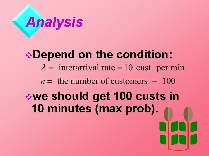
Analysis v. Depend vwe on the condition: should get 100 custs in 10 minutes (max prob).

To obtain numbers with a Poisson pdf, you can write a program: Acceptance Rejection Method

Prove: v. Poisson arrivals gene -rate an exponential interarrival pdf.

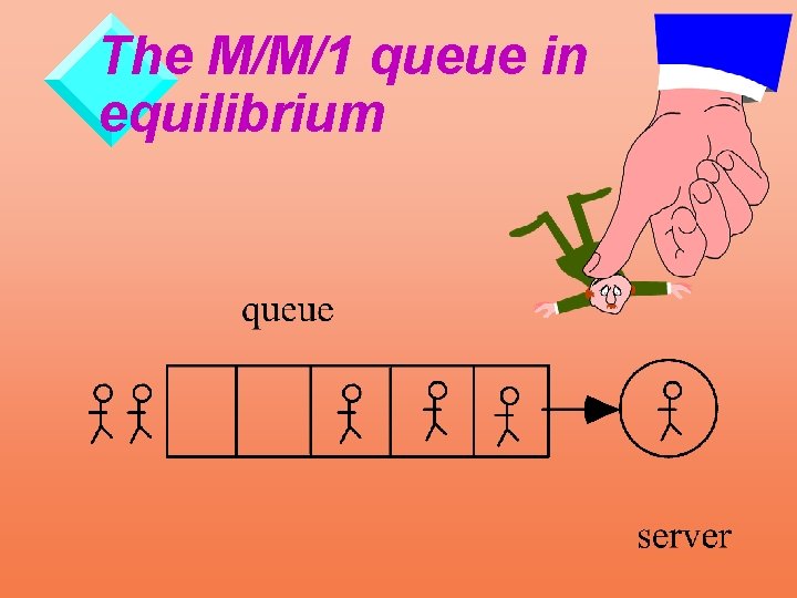
The M/M/1 queue in equilibrium

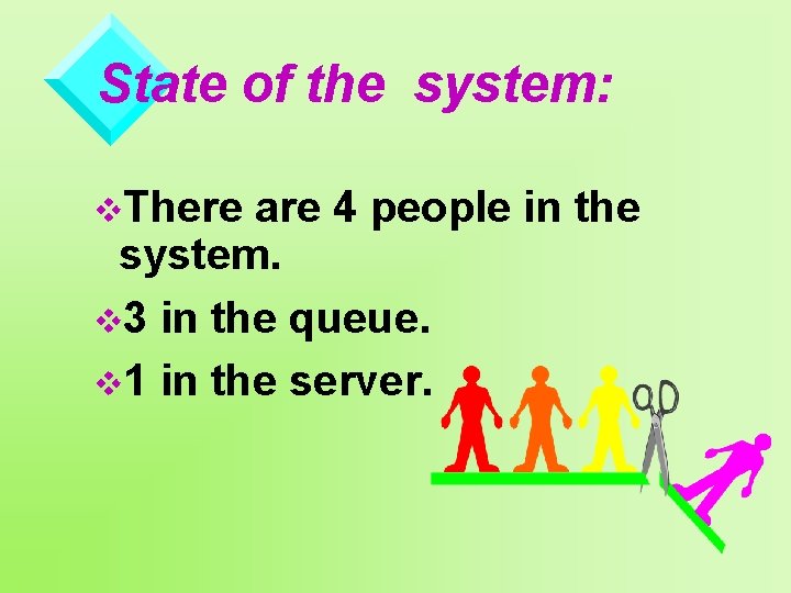
State of the system: v. There are 4 people in the system. v 3 in the queue. v 1 in the server.

Memory of M/M/1: v. The amount of time the person in the server has already spent being served is independent of the probability of the remaining service time.

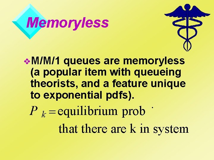
Memoryless v. M/M/1 queues are memoryless (a popular item with queueing theorists, and a feature unique to exponential pdfs). . P k = equilibrium prob that there are k in system

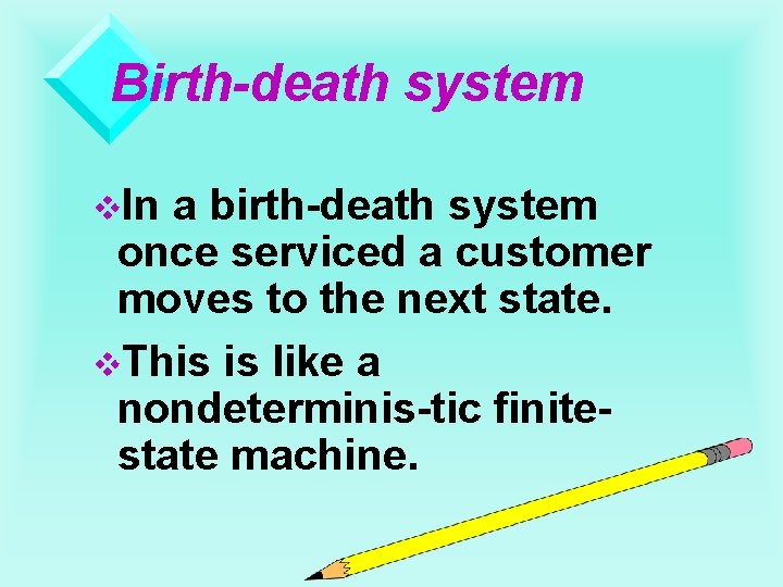
Birth-death system v. In a birth-death system once serviced a customer moves to the next state. v. This is like a nondeterminis-tic finitestate machine.

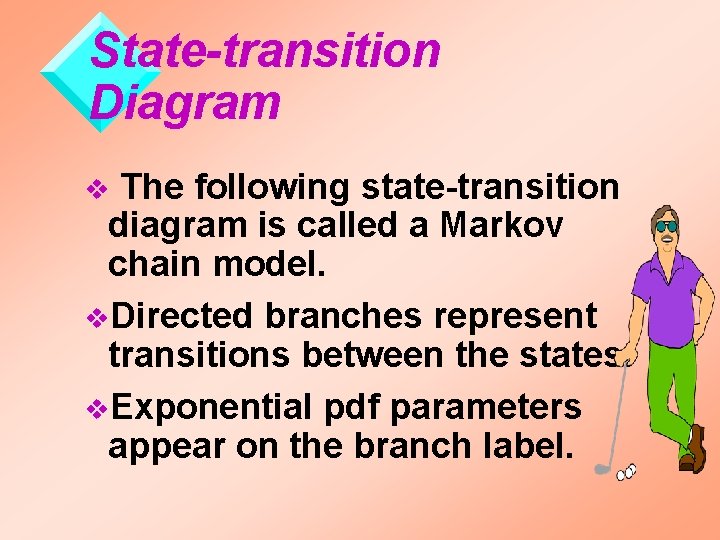
State-transition Diagram The following state-transition diagram is called a Markov chain model. v. Directed branches represent transitions between the states. v. Exponential pdf parameters appear on the branch label. v

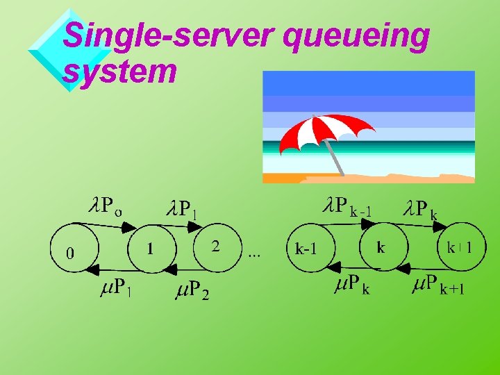
Single-server queueing system

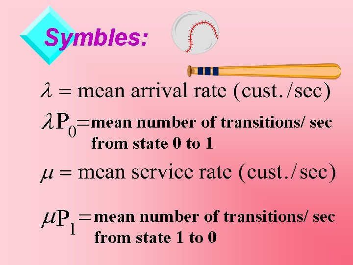
Symbles: l P 0= mean number of transitions/ sec from state 0 to 1 m P 1 = mean number of transitions/ sec from state 1 to 0

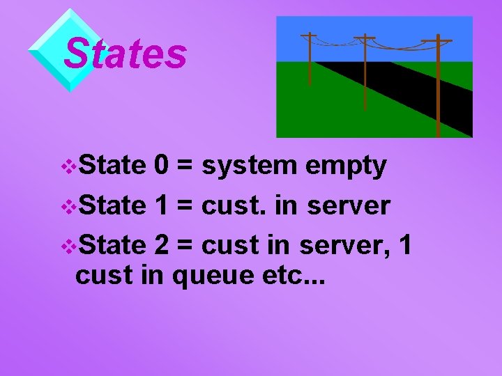
States v. State 0 = system empty v. State 1 = cust. in server v. State 2 = cust in server, 1 cust in queue etc. . .

Probalility of Given State v. Prob. of a given state is invariant if system is in equilibrium. v. The prob. of k cust’s in system is constant.

Similar to AC v. This is like AC current entering a node vis called detailed balancing vthe number leaving a node must equal the number entering

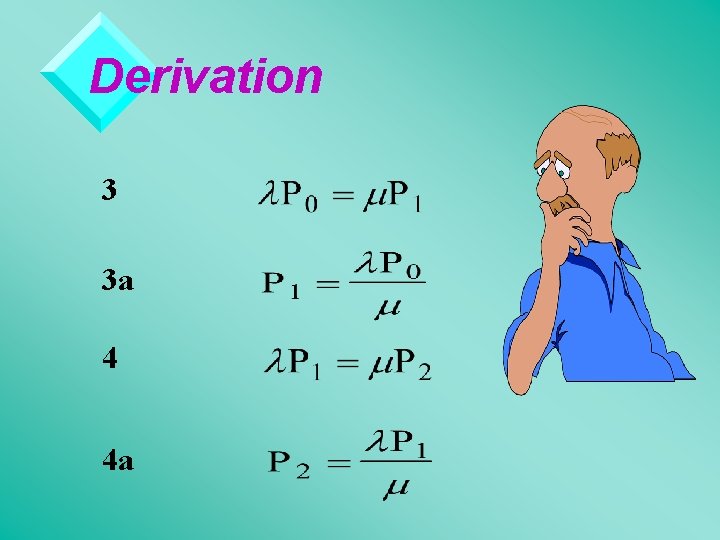
Derivation 3 3 a 4 4 a

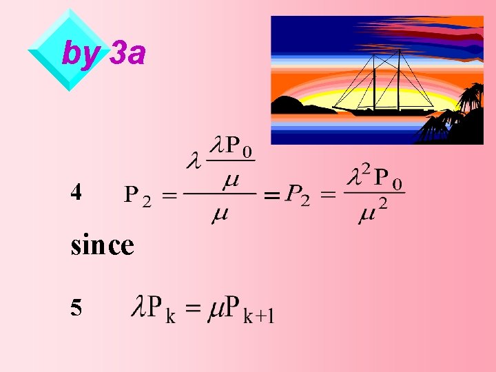
by 3 a 4 since 5 =

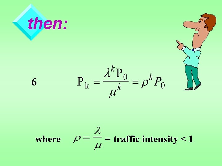
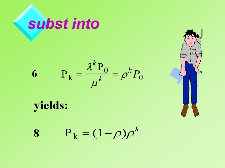
then: 6 where = traffic intensity < 1

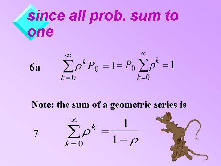
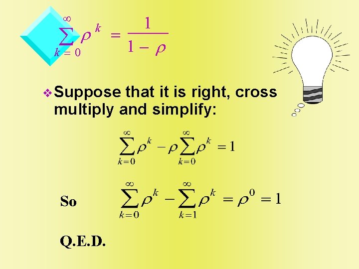
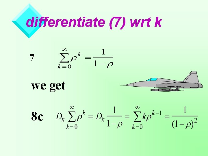
since all prob. sum to one 6 a Note: the sum of a geometric series is 7

¥ år k k=0 1 = 1 - r v. Suppose that it is right, cross multiply and simplify: So Q. E. D.

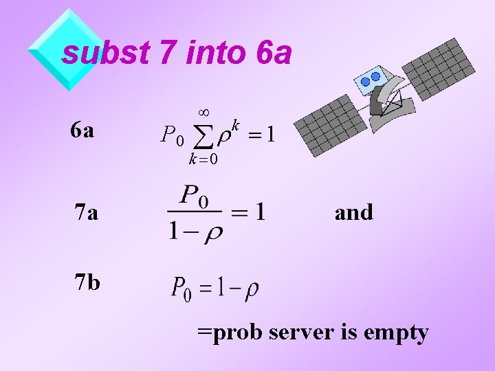
subst 7 into 6 a 6 a 7 a ¥ P 0 år k =1 k =0 and 7 b =prob server is empty

subst into 6 yields: 8

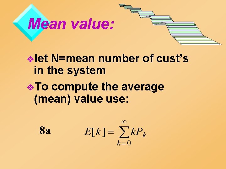
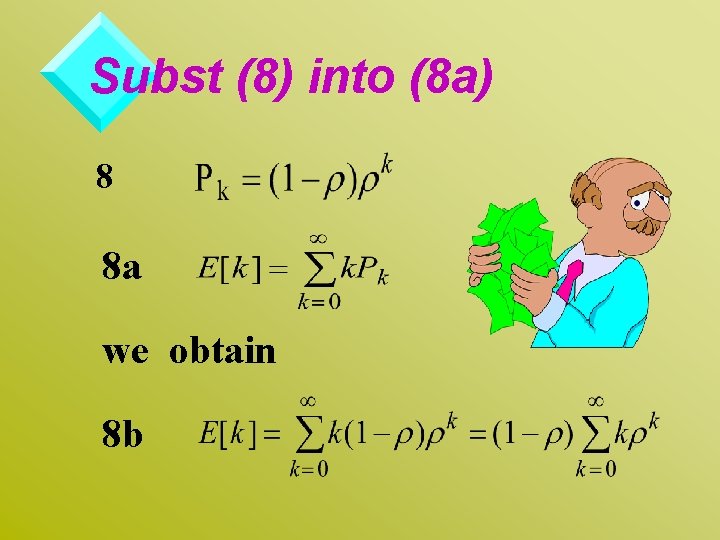
Mean value: vlet N=mean number of cust’s in the system v. To compute the average (mean) value use: 8 a

Subst (8) into (8 a) 8 8 a we obtain 8 b

differentiate (7) wrt k 7 we get 8 c

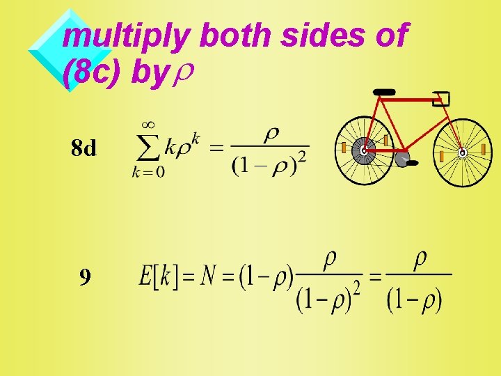
multiply both sides of (8 c) by r 8 d 9

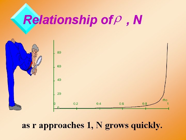
Relationship of r , N as r approaches 1, N grows quickly.

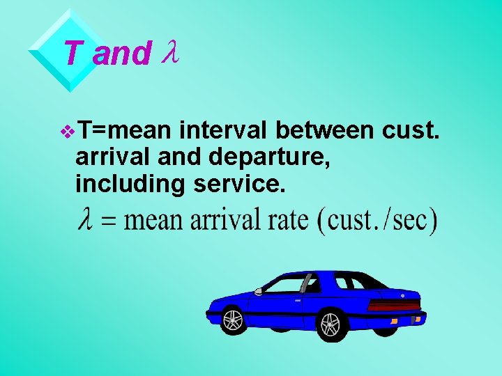
T and l v. T=mean interval between cust. arrival and departure, including service.

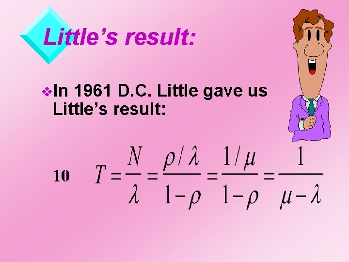
Little’s result: v. In 1961 D. C. Little gave us Little’s result: 10

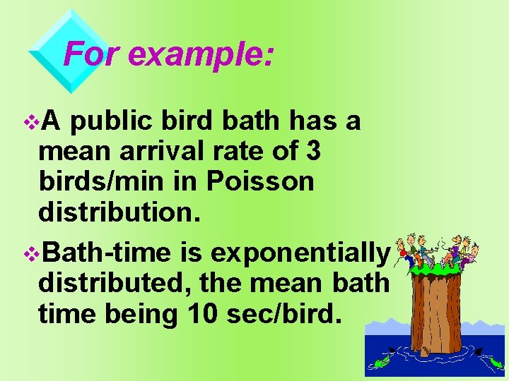
For example: v. A public bird bath has a mean arrival rate of 3 birds/min in Poisson distribution. v. Bath-time is exponentially distributed, the mean bath time being 10 sec/bird.

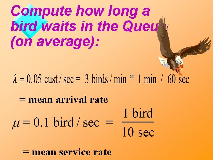
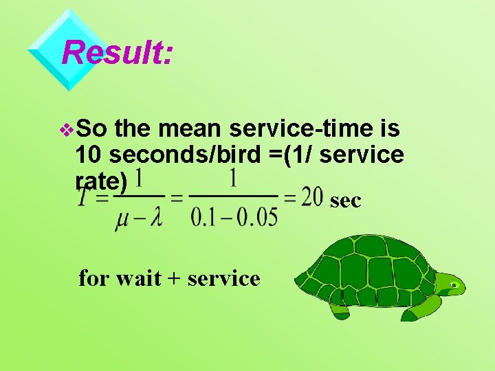
Compute how long a bird waits in the Queue (on average): = mean arrival rate = mean service rate

Result: v. So the mean service-time is 10 seconds/bird =(1/ service rate) sec for wait + service

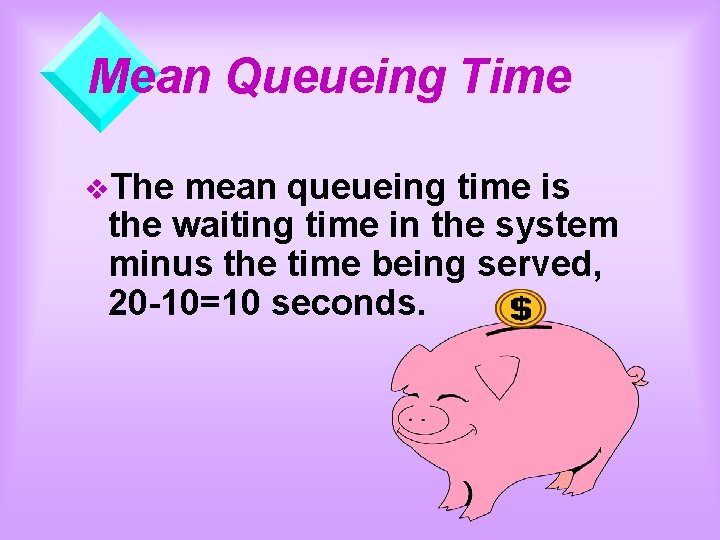
Mean Queueing Time v. The mean queueing time is the waiting time in the system minus the time being served, 20 -10=10 seconds.

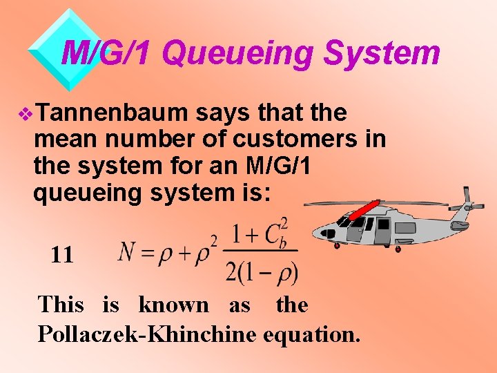
M/G/1 Queueing System v. Tannenbaum says that the mean number of customers in the system for an M/G/1 queueing system is: 11 This is known as the Pollaczek-Khinchine equation.

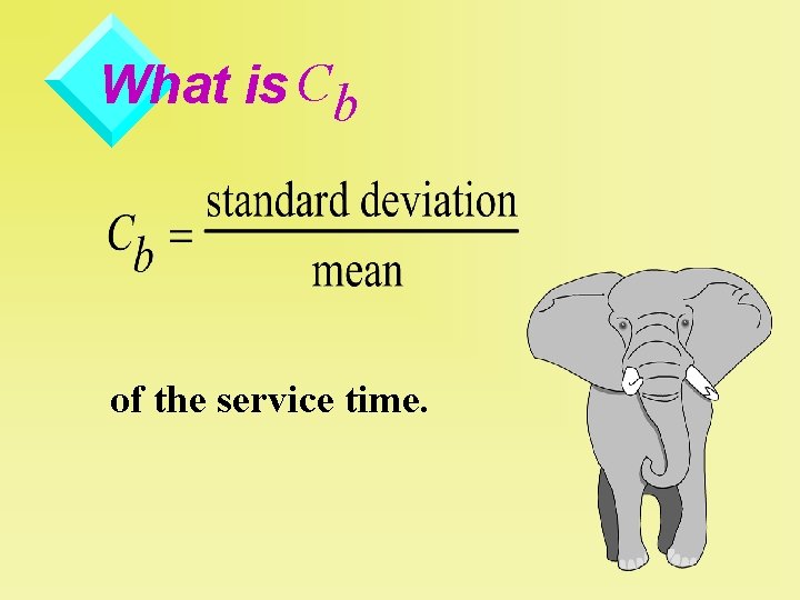
What is Cb of the service time.

Note: v. M/G/1 means that it is valid for any service-time distribution. v. For identical service time means, the large standard deviation will give a longer service time.

Thanking You…!!