Introduction to Quantum Information Processing QIC 710 CS

Introduction to Quantum Information Processing QIC 710 / CS 768 / PH 767 / CO 681 / AM 871 Lectures 10– 11 (2019) Richard Cleve QNC 3129 cleve@uwaterloo. ca 1 © Richard Cleve 2020

More state distinguishing problems 2 © Richard Cleve 2020

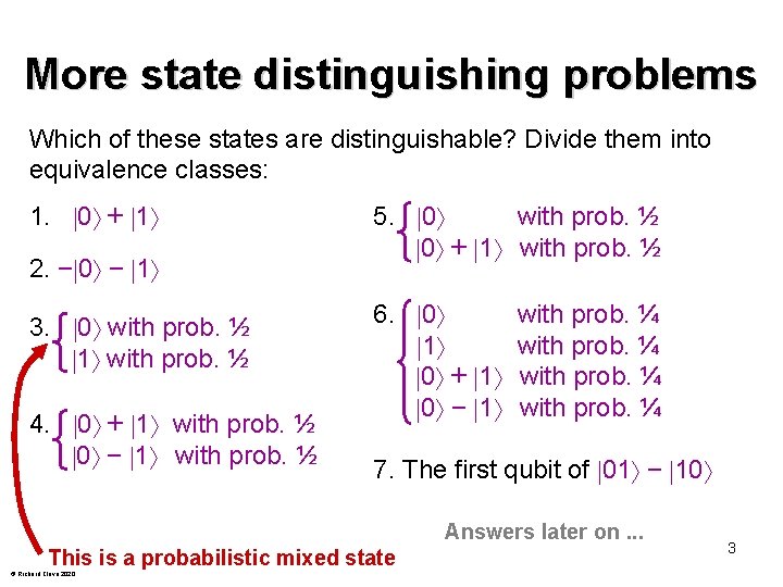
More state distinguishing problems Which of these states are distinguishable? Divide them into equivalence classes: 1. 0 + 1 2. − 0 − 1 3. 0 with prob. ½ 1 with prob. ½ 4. 0 + 1 with prob. ½ 0 − 1 with prob. ½ 5. 0 with prob. ½ 0 + 1 with prob. ½ 6. 0 1 0 + 1 0 − 1 with prob. ¼ 7. The first qubit of 01 − 10 Answers later on. . . This is a probabilistic mixed state © Richard Cleve 2020 3

Density matrix formalism 4 © Richard Cleve 2020

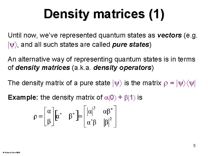
Density matrices (1) Until now, we’ve represented quantum states as vectors (e. g. ψ , and all such states are called pure states) An alternative way of representing quantum states is in terms of density matrices (a. k. a. density operators) The density matrix of a pure state ψ is the matrix = ψ ψ Example: the density matrix of 0 + 1 is 5 © Richard Cleve 2020

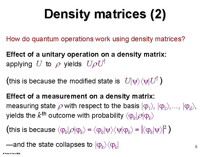
Density matrices (2) How do quantum operations work using density matrices? Effect of a unitary operation on a density matrix: † applying U to yields U U (this is because the modified state is U ψ ψ U† ) Effect of a measurement on a density matrix: measuring state with respect to the basis 1 , 2 , . . . , d , yields the k th outcome with probability k k (this is because k k = k ψ ψ k = k ψ 2 ) —and the state collapses to k k © Richard Cleve 2020 6

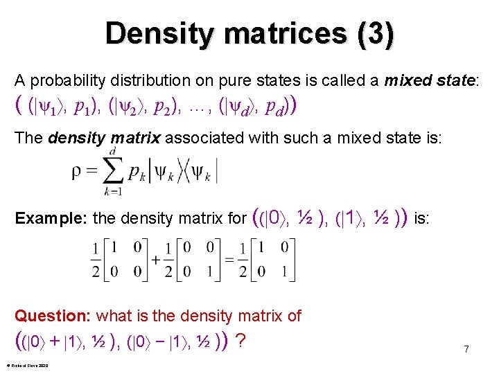
Density matrices (3) A probability distribution on pure states is called a mixed state: ( ( ψ1 , p 1), ( ψ2 , p 2), …, ( ψd , pd)) The density matrix associated with such a mixed state is: Example: the density matrix for (( 0 , ½ ), ( 1 , ½ )) is: Question: what is the density matrix of (( 0 + 1 , ½ ), ( 0 − 1 , ½ )) ? © Richard Cleve 2020 7

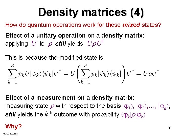
Density matrices (4) How do quantum operations work for these mixed states? Effect of a unitary operation on a density matrix: † applying U to still yields U U This is because the modified state is: Effect of a measurement on a density matrix: measuring state with respect to the basis 1 , 2 , . . . , d , still yields the k th outcome with probability k k Why? © Richard Cleve 2020 8

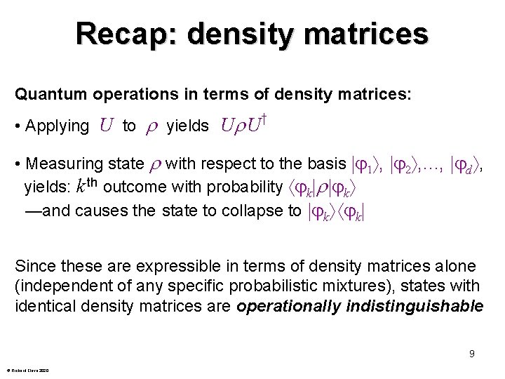
Recap: density matrices Quantum operations in terms of density matrices: • Applying U to yields U U† • Measuring state with respect to the basis 1 , 2 , . . . , d , yields: k th outcome with probability k k —and causes the state to collapse to k k Since these are expressible in terms of density matrices alone (independent of any specific probabilistic mixtures), states with identical density matrices are operationally indistinguishable 9 © Richard Cleve 2020

Return to state distinguishing problems … 10 © Richard Cleve 2020

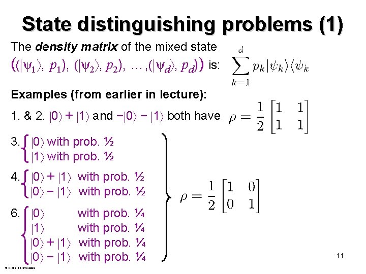
State distinguishing problems (1) The density matrix of the mixed state (( ψ1 , p 1), ( ψ2 , p 2), …, ( ψd , pd)) is: Examples (from earlier in lecture): 1. & 2. 0 + 1 and − 0 − 1 both have 3. 0 with prob. ½ 1 with prob. ½ 4. 0 + 1 with prob. ½ 0 − 1 with prob. ½ 6. 0 1 0 + 1 0 − 1 © Richard Cleve 2020 with prob. ¼ 11

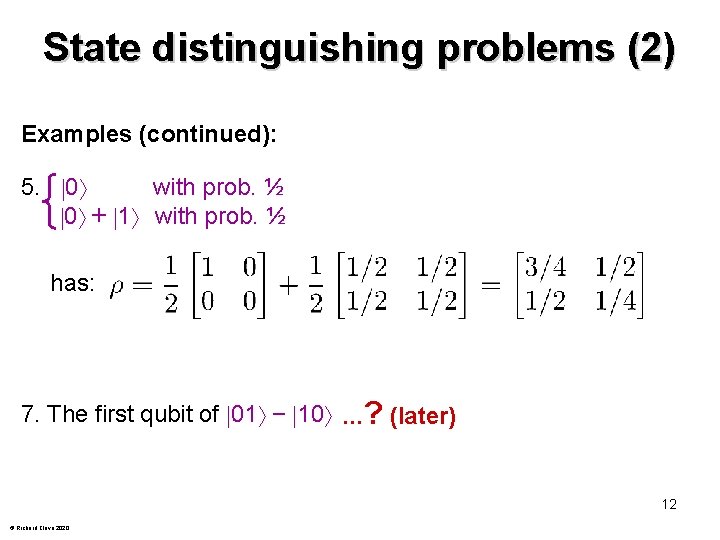
State distinguishing problems (2) Examples (continued): 5. 0 with prob. ½ 0 + 1 with prob. ½ has: 7. The first qubit of 01 − 10 . . . ? (later) 12 © Richard Cleve 2020

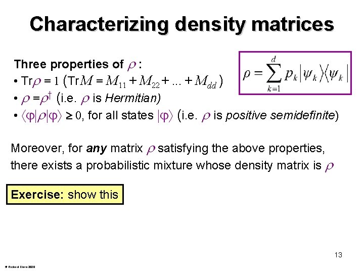
Characterizing density matrices Three properties of : • Tr = 1 (Tr M = M 11 + M 22 +. . . + Mdd ) • = † (i. e. is Hermitian) • 0, for all states (i. e. is positive semidefinite) Moreover, for any matrix satisfying the above properties, there exists a probabilistic mixture whose density matrix is Exercise: show this 13 © Richard Cleve 2020

Taxonomy of various normal matrices 14 © Richard Cleve 2020

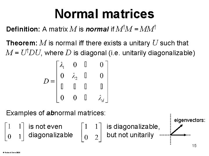
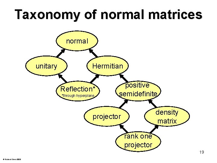
Normal matrices Definition: A matrix M is normal if M†M = MM† Theorem: M is normal iff there exists a unitary U such that M = U†DU, where D is diagonal (i. e. unitarily diagonalizable) Examples of abnormal matrices: is not even diagonalizable is diagonalizable, but not unitarily eigenvectors: 15 © Richard Cleve 2020

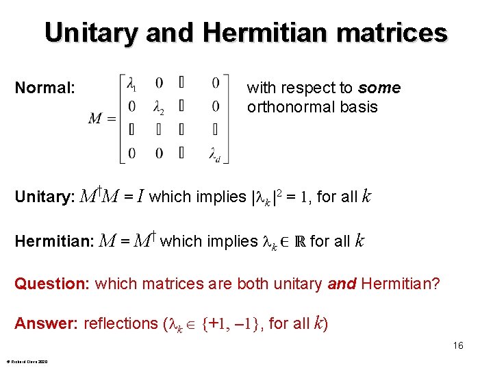
Unitary and Hermitian matrices Normal: with respect to some orthonormal basis Unitary: M†M = I which implies | k |2 = 1, for all k Hermitian: M = M† which implies k ∈ ℝ for all k Question: which matrices are both unitary and Hermitian? Answer: reflections ( k {+1, – 1}, for all k) 16 © Richard Cleve 2020

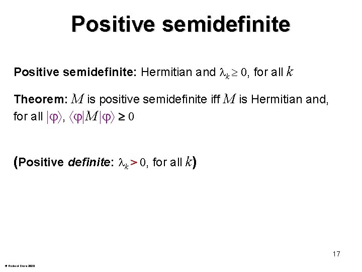
Positive semidefinite: Hermitian and k 0, for all k Theorem: M is positive semidefinite iff M is Hermitian and, for all , M 0 (Positive definite: k > 0, for all k) 17 © Richard Cleve 2020

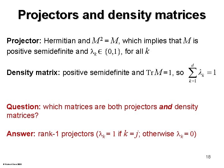
Projectors and density matrices Projector: Hermitian and M 2 = M, which implies that M is positive semidefinite and k ∈ {0, 1}, for all k Density matrix: positive semidefinite and Tr M = 1, so Question: which matrices are both projectors and density matrices? Answer: rank-1 projectors ( k = 1 if k = j; otherwise k = 0) 18 © Richard Cleve 2020

Taxonomy of normal matrices normal unitary Hermitian Reflection* *through hyperplane positive semidefinite density matrix projector rank one projector 19 © Richard Cleve 2020

Bloch sphere for qubits 20 © Richard Cleve 2020

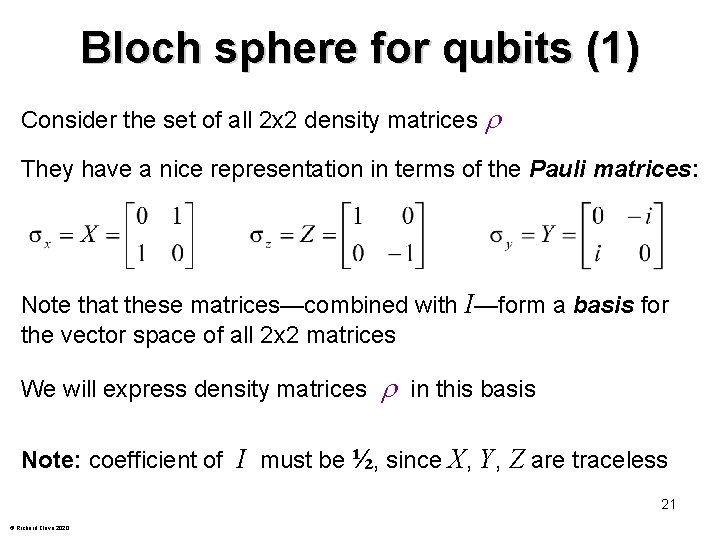
Bloch sphere for qubits (1) Consider the set of all 2 x 2 density matrices They have a nice representation in terms of the Pauli matrices: Note that these matrices—combined with I—form a basis for the vector space of all 2 x 2 matrices We will express density matrices in this basis Note: coefficient of I must be ½, since X, Y, Z are traceless 21 © Richard Cleve 2020

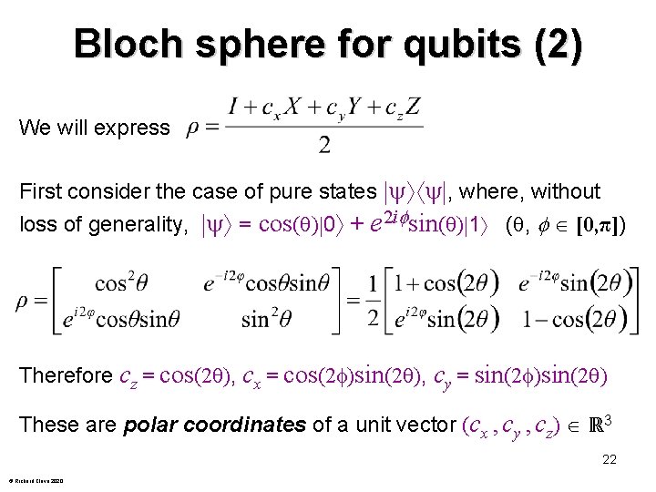
Bloch sphere for qubits (2) We will express First consider the case of pure states , where, without loss of generality, = cos( ) 0 + e 2 i sin( ) 1 ( , [0, π]) Therefore cz = cos(2 ), cx = cos(2 )sin(2 ), cy = sin(2 ) These are polar coordinates of a unit vector (cx , cy , cz) ℝ 3 22 © Richard Cleve 2020

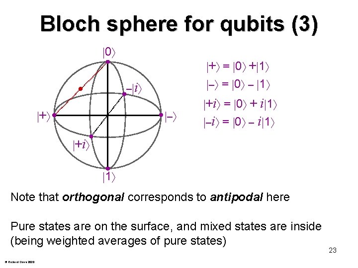
Bloch sphere for qubits (3) 0 + = 0 + 1 – = 0 – 1 – i + – +i = 0 + i 1 –i = 0 – i 1 +i 1 Note that orthogonal corresponds to antipodal here Pure states are on the surface, and mixed states are inside (being weighted averages of pure states) © Richard Cleve 2020 23

Distinguishing mixed states 24 © Richard Cleve 2020

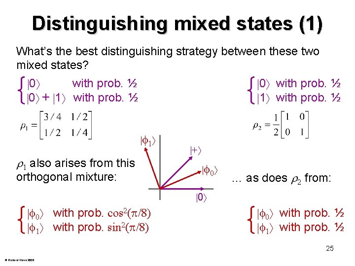
Distinguishing mixed states (1) What’s the best distinguishing strategy between these two mixed states? 0 with prob. ½ 1 with prob. ½ 0 with prob. ½ 0 + 1 with prob. ½ 1 1 also arises from this orthogonal mixture: + 0 … as does 2 from: 0 0 with prob. cos 2( /8) 1 with prob. sin 2( /8) 0 with prob. ½ 1 with prob. ½ 25 © Richard Cleve 2020

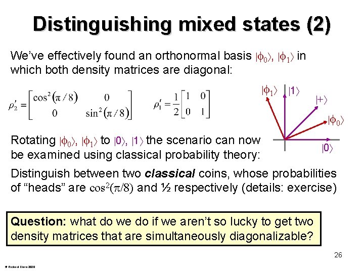
Distinguishing mixed states (2) We’ve effectively found an orthonormal basis 0 , 1 in which both density matrices are diagonal: 1 1 + 0 Rotating 0 , 1 to 0 , 1 the scenario can now be examined using classical probability theory: 0 Distinguish between two classical coins, whose probabilities of “heads” are cos 2( /8) and ½ respectively (details: exercise) Question: what do we do if we aren’t so lucky to get two density matrices that are simultaneously diagonalizable? 26 © Richard Cleve 2020

general quantum operations more commonly known as quantum channels 27 © Richard Cleve 2020

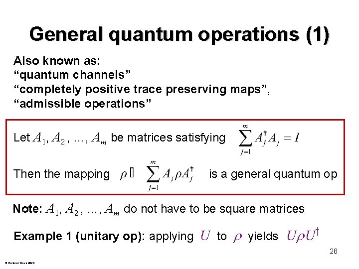
General quantum operations (1) Also known as: “quantum channels” “completely positive trace preserving maps”, “admissible operations” Let A 1, A 2 , …, Am be matrices satisfying Then the mapping is a general quantum op Note: A 1, A 2 , …, Am do not have to be square matrices Example 1 (unitary op): applying U to yields U U† 28 © Richard Cleve 2020

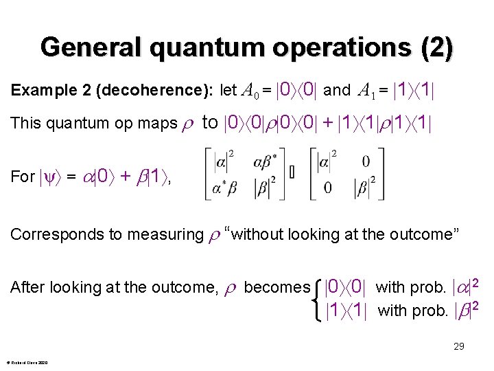
General quantum operations (2) Example 2 (decoherence): let A 0 = 0 0 and A 1 = 1 1 This quantum op maps to 0 0 + 1 1 For ψ = 0 + 1 , Corresponds to measuring “without looking at the outcome” After looking at the outcome, becomes 0 0 with prob. | |2 1 1 with prob. | |2 29 © Richard Cleve 2020

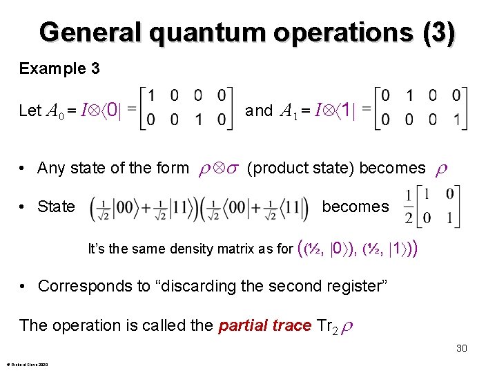
General quantum operations (3) Example 3 Let A 0 = I 0 • Any state of the form • State and A 1 = I 1 (product state) becomes It’s the same density matrix as for ((½ , 0 ), (½ , 1 )) • Corresponds to “discarding the second register” The operation is called the partial trace Tr 2 30 © Richard Cleve 2020