Introduction to Quantum Information Processing CS 467 CS

Introduction to Quantum Information Processing CS 467 / CS 667 Phys 667 / Phys 767 C&O 481 / C&O 681 Lecture 7 (2008) Richard Cleve DC 2117 cleve@cs. uwaterloo. ca 1

Definition of the quantum Fourier transform (QFT) 2

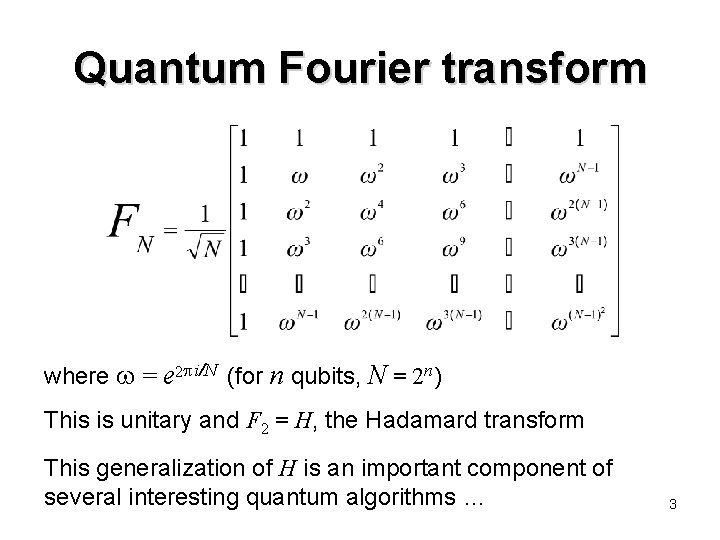
Quantum Fourier transform where = e 2 i/N (for n qubits, N = 2 n) This is unitary and F 2 = H, the Hadamard transform This generalization of H is an important component of several interesting quantum algorithms … 3

Discrete log problem 4

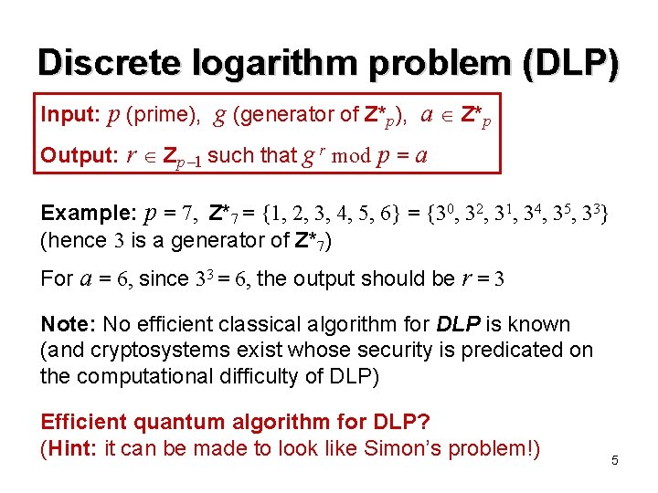
Discrete logarithm problem (DLP) Input: p (prime), g (generator of Z*p), a Z*p Output: r Zp 1 such that g r mod p = a Example: p = 7, Z*7 = {1, 2, 3, 4, 5, 6} = {30, 32, 31, 34, 35, 33} (hence 3 is a generator of Z*7) For a = 6, since 33 = 6, the output should be r = 3 Note: No efficient classical algorithm for DLP is known (and cryptosystems exist whose security is predicated on the computational difficulty of DLP) Efficient quantum algorithm for DLP? (Hint: it can be made to look like Simon’s problem!) 5

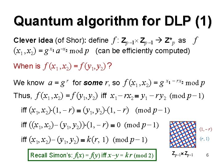
Quantum algorithm for DLP (1) Clever idea (of Shor): define f : Zp 1 Z*p as f (x 1 , x 2) = g x 1 a x 2 mod p (can be efficiently computed) When is f (x 1 , x 2) = f (y 1, y 2) ? We know a = g r for some r, so f (x 1 , x 2) = g x 1 r x 2 mod p Thus, f (x 1 , x 2) = f (y 1, y 2) iff x 1 rx 2 y 1 r y 2 (mod p 1) iff (x 1, x 2) (1, r) (y 1, y 2) (1, r) (mod p 1) iff ((x 1, x 2) (y 1, y 2)) (1, r) 0 (mod p 1) (1, r) iff (x 1, x 2) (y 1, y 2) k (r, 1) (mod p 1) Recall Simon’s: f(x) = f(y) iff x y = k r (mod 2) (r, 1) Zp 1 6

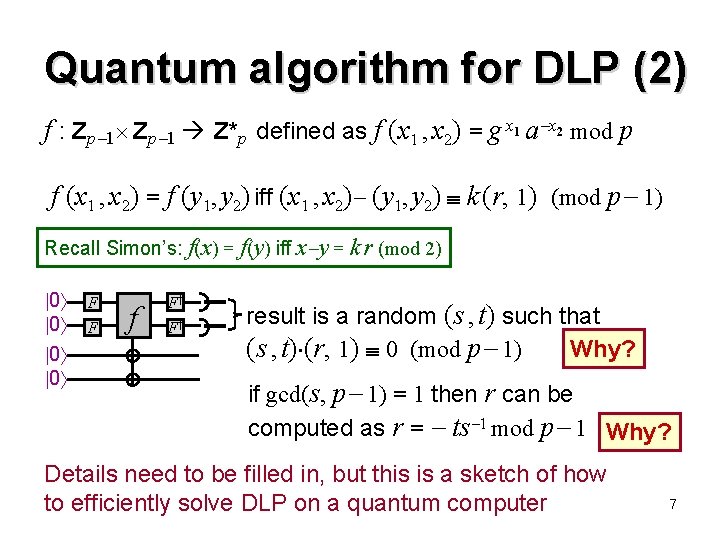
Quantum algorithm for DLP (2) f : Zp 1 Z*p defined as f (x 1 , x 2) = g x 1 a x 2 mod p f (x 1 , x 2) = f (y 1, y 2) iff (x 1 , x 2) (y 1, y 2) k (r, 1) (mod p 1) Recall Simon’s: f(x) = f(y) iff x y = k r (mod 2) 0 0 F F f F† F† result is a random (s , t) such that Why? (s , t) (r, 1) 0 (mod p 1) if gcd(s, p 1) = 1 then r can be computed as r = ts 1 mod p 1 Why? Details need to be filled in, but this is a sketch of how to efficiently solve DLP on a quantum computer 7

Introduction to Quantum Information Processing CS 467 / CS 667 Phys 667 / Phys 767 C&O 481 / C&O 681 Lecture 8 (2008) Richard Cleve DC 2117 cleve@cs. uwaterloo. ca 8

Computing the QFT n for N = 2 9

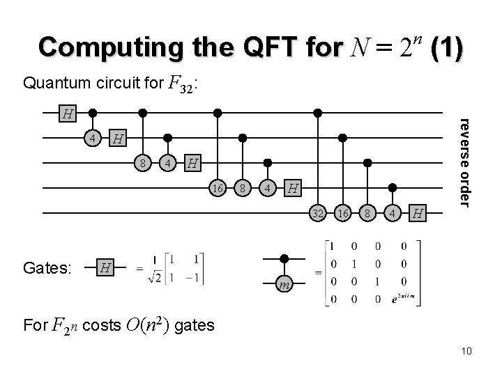
n Computing the QFT for N = 2 (1) Quantum circuit for F 32: H 4 8 4 H 16 8 4 H 32 Gates: 16 8 4 H reverse order H H m For F 2 n costs O(n 2) gates 10

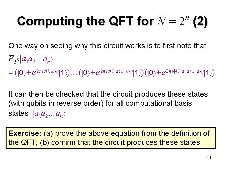
n Computing the QFT for N = 2 (2) One way on seeing why this circuit works is to first note that F 2 n a 1 a 2…an = ( 0 + e 2 i (0. an) 1 )…( 0 + e 2 i (0. a 2…an) 1 ) ( 0 + e 2 i (0. a 1 a 2…an) 1 ) It can then be checked that the circuit produces these states (with qubits in reverse order) for all computational basis states a 1 a 2…an Exercise: (a) prove the above equation from the definition of the QFT; (b) confirm that the circuit produces these states 11

Contents Loose ends in the discrete log algorithm 12

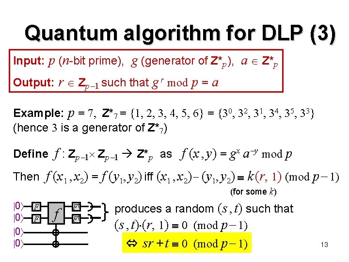
Quantum algorithm for DLP (3) Input: p (n-bit prime), g (generator of Z*p), a Z*p Output: r Zp 1 such that g r mod p = a Example: p = 7, Z*7 = {1, 2, 3, 4, 5, 6} = {30, 32, 31, 34, 35, 33} (hence 3 is a generator of Z*7) Define f : Zp 1 Z*p as f (x , y) = gx a y mod p Then f (x 1 , x 2) = f (y 1, y 2) iff (x 1 , x 2) (y 1, y 2) k (r, 1) (mod p 1) (for some k) 0 0 F F f F† F† produces a random (s , t) such that (s , t) (r, 1) 0 (mod p 1) sr + t 0 (mod p 1) 13

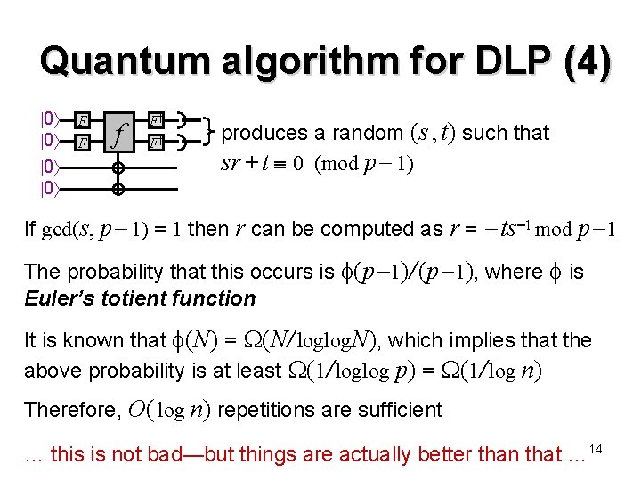
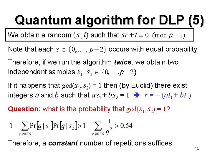
Quantum algorithm for DLP (4) 0 0 F F f F† F† produces a random (s , t) such that sr + t 0 (mod p 1) If gcd(s, p 1) = 1 then r can be computed as r = ts 1 mod p 1 The probability that this occurs is (p 1)/ (p 1), where is Euler’s totient function It is known that (N) = (N/ loglog. N), which implies that the above probability is at least (1/ loglog p) = (1/ log n) Therefore, O( log n) repetitions are sufficient … this is not bad—but things are actually better than that … 14

Quantum algorithm for DLP (5) We obtain a random (s , t) such that sr + t 0 (mod p 1) Note that each s {0, …, p 2} occurs with equal probability Therefore, if we run the algorithm twice: we obtain two independent samples s 1, s 2 {0, …, p 2} If it happens that gcd(s 1, s 2) = 1 then (by Euclid) there exist integers a and b such that as 1 + bs 2 = 1 r = (at 1 + bt 2) Question: what is the probability that gcd(s 1, s 2) = 1? Therefore, a constant number of repetitions suffices 15

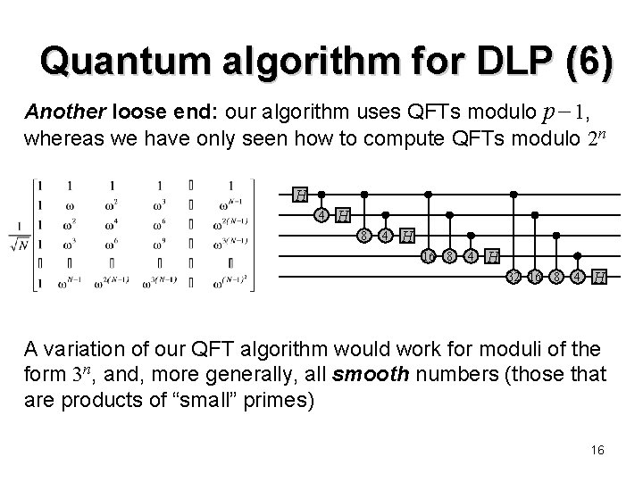
Quantum algorithm for DLP (6) Another loose end: our algorithm uses QFTs modulo p 1, whereas we have only seen how to compute QFTs modulo 2 n H 4 H 8 4 H 16 8 4 H 32 16 8 4 H A variation of our QFT algorithm would work for moduli of the form 3 n, and, more generally, all smooth numbers (those that are products of “small” primes) 16

Quantum algorithm for DLP (7) In fact, for the case where p 1 is smooth, there already exist polynomial-time classical algorithms for discrete log! It’s only the case where p 1 is not smooth that is interesting Shor just used a modulus close to p 1, and, using careful error-analysis, showed that this was good enough. . . There also ways of attaining good approximations of QFTs for arbitrary moduli—which we will see later on (so this loose end is not yet resolved) 17

On simulating black boxes 18

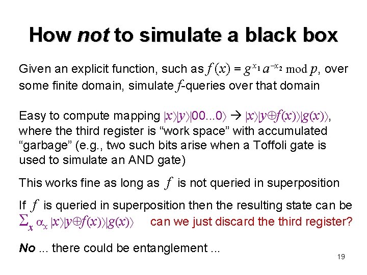
How not to simulate a black box Given an explicit function, such as f (x) = g x 1 a x 2 mod p, over some finite domain, simulate f-queries over that domain Easy to compute mapping x y 00. . . 0 x y f (x) g(x) , where third register is “work space” with accumulated “garbage” (e. g. , two such bits arise when a Toffoli gate is used to simulate an AND gate) This works fine as long as f is not queried in superposition If f is queried in superposition the resulting state can be x x x y f (x) g(x) can we just discard the third register? No. . . there could be entanglement. . . 19

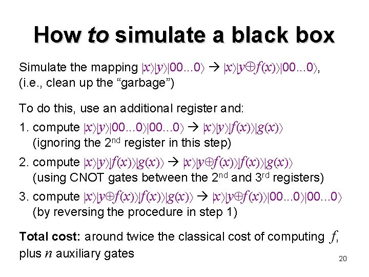
How to simulate a black box Simulate the mapping x y 00. . . 0 x y f (x) 00. . . 0 , (i. e. , clean up the “garbage”) To do this, use an additional register and: 1. compute x y 00. . . 0 x y f (x) g(x) (ignoring the 2 nd register in this step) 2. compute x y f (x) g(x) (using CNOT gates between the 2 nd and 3 rd registers) 3. compute x y f (x) g(x) x y f (x) 00. . . 0 (by reversing the procedure in step 1) Total cost: around twice the classical cost of computing f, plus n auxiliary gates 20

The “hidden subgroup” framework 21

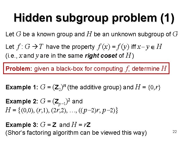
Hidden subgroup problem (1) Let G be a known group and H be an unknown subgroup of G Let f : G T have the property f (x) = f (y) iff x y H (i. e. , x and y are in the same right coset of H ) Problem: given a black-box for computing f, determine H Example 1: G = (Z 2)n (the additive group) and H = {0, r} Example 2: G = (Zp 1)2 and H = {(0, 0), (r, 1), (2 r, 2), …, (( p 2)r, p 2)} Example 3: G = Z and H = r. Z (Shor’s factoring algorithm can be viewed this way) 22

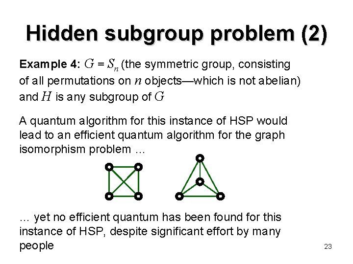
Hidden subgroup problem (2) Example 4: G = Sn (the symmetric group, consisting of all permutations on n objects—which is not abelian) and H is any subgroup of G A quantum algorithm for this instance of HSP would lead to an efficient quantum algorithm for the graph isomorphism problem … … yet no efficient quantum has been found for this instance of HSP, despite significant effort by many people 23

Introduction to Quantum Information Processing CS 467 / CS 667 Phys 667 / Phys 767 C&O 481 / C&O 681 Lecture 9 (2008) Richard Cleve DC 2117 cleve@cs. uwaterloo. ca 24

Eigenvalue estimation problem (a. k. a. phase estimation) Note: this is a major component of Shor’s factoring algorithm 25

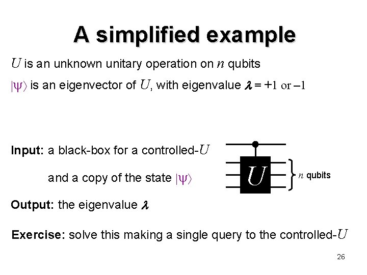
A simplified example U is an unknown unitary operation on n qubits is an eigenvector of U, with eigenvalue = +1 or – 1 Input: a black-box for a controlled-U and a copy of the state U n qubits Output: the eigenvalue Exercise: solve this making a single query to the controlled-U 26

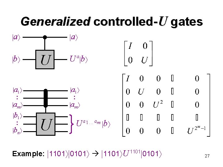
Generalized controlled-U gates a b a U a 1 : am b 1 : bn U a b a 1 : am U U a 1 am b Example: 1101 0101 1101 U 1101 0101 27

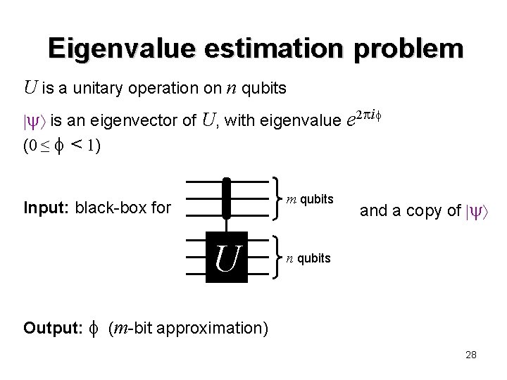
Eigenvalue estimation problem U is a unitary operation on n qubits is an eigenvector of U, with eigenvalue e 2 i (0 ≤ < 1) m qubits Input: black-box for U and a copy of n qubits Output: (m-bit approximation) 28

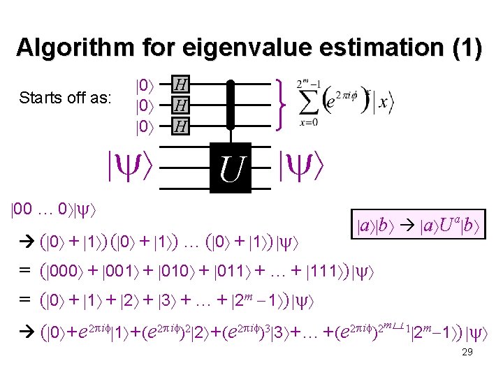
Algorithm for eigenvalue estimation (1) Starts off as: 0 0 0 H H H U 00 … 0 ( 0 + 1 ) … ( 0 + 1 ) a b a U a b = ( 000 + 001 + 010 + 011 + … + 111 ) = ( 0 + 1 + 2 + 3 + … + 2 m 1 ) ( 0 + e 2 i 1 + (e 2 i )2 2 + (e 2 i )3 3 + … + (e 2 i )2 2 m 1 ) m� 1 29

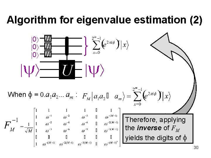
Algorithm for eigenvalue estimation (2) 0 H 0 H U When = 0. a 1 a 2…am : Therefore, applying the inverse of FM yields the digits of 30

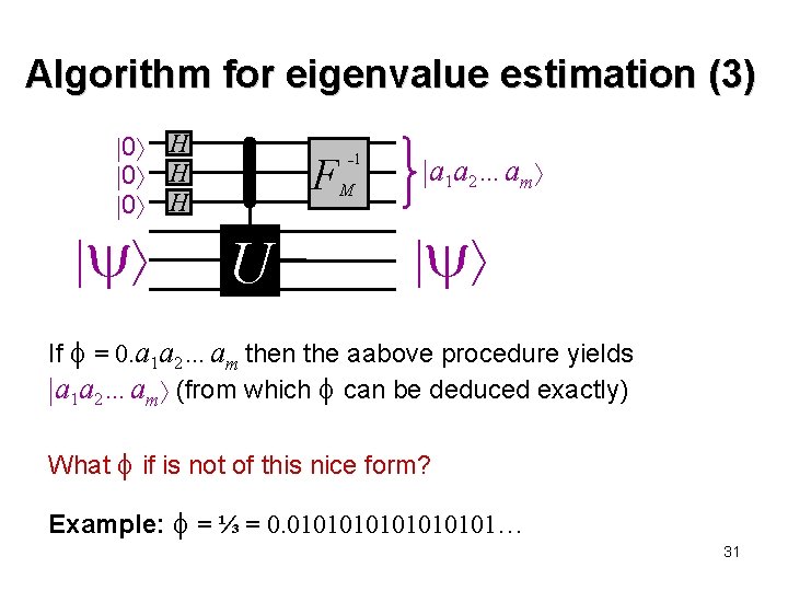
Algorithm for eigenvalue estimation (3) 0 H 0 H F U – 1 M a 1 a 2…am If = 0. a 1 a 2…am then the aabove procedure yields a 1 a 2…am (from which can be deduced exactly) What if is not of this nice form? Example: = ⅓ = 0. 01010101… 31

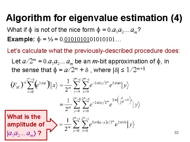
Algorithm for eigenvalue estimation (4) What if is not of the nice form = 0. a 1 a 2…am? Example: = ⅓ = 0. 01010101… Let’s calculate what the previously-described procedure does: Let a / 2 m = 0. a 1 a 2…am be an m-bit approximation of , in the sense that = a / 2 m + , where | | ≤ 1 / 2 m+1 What is the amplitude of a 1 a 2…am ? 32

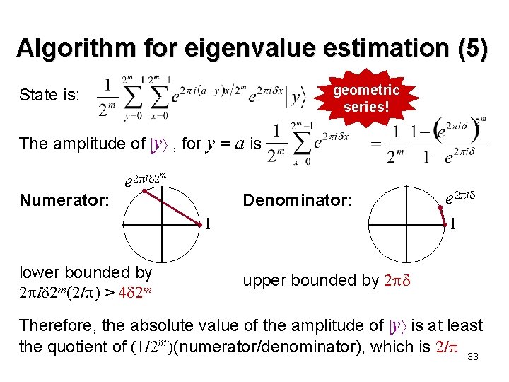
Algorithm for eigenvalue estimation (5) geometric series! State is: The amplitude of y , for y = a is Numerator: e 2 i 2 m Denominator: 1 1 lower bounded by 2 i 2 m(2/ ) > 4 2 m e 2 i upper bounded by 2 Therefore, the absolute value of the amplitude of y is at least the quotient of (1/2 m)(numerator/denominator), which is 2/ 33

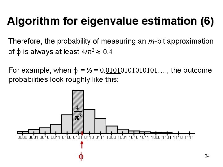
Algorithm for eigenvalue estimation (6) Therefore, the probability of measuring an m-bit approximation of is always at least 4/ 2 0. 4 For example, when = ⅓ = 0. 01010101… , the outcome probabilities look roughly like this: 4 2 0000 0001 0010 0011 0100 0101 0110 0111 1000 1001 1010 1011 1000 1101 1110 1111 34