Introduction to Python An Introduction to Numpy Topics

Introduction to Python An Introduction to Numpy

Topics 1) Numpy

Numpy Python is currently one of most popular languages for data science and machine learning. In the next set of lectures, we will focus on working with and analyzing data. Python has many optimized libraries for working with data. We will cover two powerful libraries for scientific computing and data processing: Numpy and pandas.

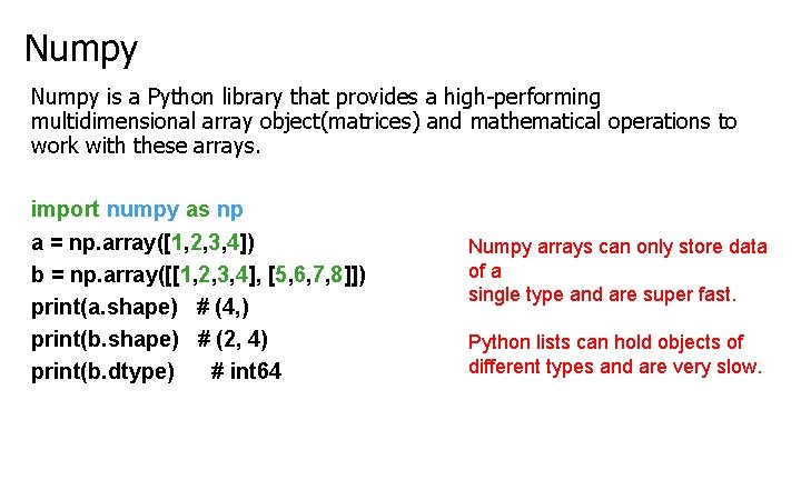
Numpy is a Python library that provides a high-performing multidimensional array object(matrices) and mathematical operations to work with these arrays. import numpy as np a = np. array([1, 2, 3, 4]) b = np. array([[1, 2, 3, 4], [5, 6, 7, 8]]) print(a. shape) # (4, ) print(b. shape) # (2, 4) print(b. dtype) # int 64 Numpy arrays can only store data of a single type and are super fast. Python lists can hold objects of different types and are very slow.

Numpy import numpy as np a = np. array([[1, 2, 3, 4], [5, 6, 7, 8], [9, 10, 11, 12]]) print(a[0, 0]) # 1 print(a[1, 3] # 8 print(a[: , 1: 3]) [[ 2, 3], [ 6, 7], [10, 11]] Note the use of commas, if it was a 2 D Python list: print(a[0][0]) Numpy uses commas(tuples) for indexing. # all rows, columns 1 and 2. Similar to Python lists, slicing works with Numpy arrays!

arange(integer ranges) import numpy as np In[5]: np. arange(5) Out[5]: array([0, 1, 2, 3, 4]) In[5]: np. arange(5, 10) Out[5]: array([5, 6, 7, 8, 9]) In[5]: np. arange(5) Out[5]: array([0, 1, 2, 3, 4]) In[5]: np. arange(7, 1, -2) Out[5]: array([7, 5, 3])

linspace(floating-point ranges) and reshape import numpy as np In[5]: np. linspace(0. 0, 1. 0, num=5) Out[5]: array([0. , 0. 25, 0. 5 , 0. 75, 1. ]) In[5]: np. arange(6). reshape(2, 3) Out[6]: array([[0, 1, 2], [3, 4, 5]])

zeros and ones import numpy as np In[5]: np. zeros((3, 2)) Out[7]: array([[0. , 0. ], [0. , 0. ]]) In[5]: np. ones((3, 2), dtype=int 64) Out[7]: array([[0, 0], [0, 0]])

Numpy Operators import numpy as np In[1]: numbers = np. arange(6). reshape(2, 3) In[2]: numbers Out[2]: array([[0, 1, 2], [3, 4, 5]]) In[3]: numbers * 2 Out[3]: array([[0, 2, 4], [6, 8, 10]]) Note that numbers is unchanged! In[4]: numbers Out[4]: array([[0, 1, 2], [3, 4, 5]])

Numpy Operators import numpy as np In[5]: numbers ** 3 Out[5]: array([[ 0, 1, 8], [ 27, 64, 125]]) In[5]: numbers += 5 In[6]: numbers Out[6]: array([[ 5, 6, 7], [ 8, 9, 10]]) Note that numbers is changed!

Numpy Operators import numpy as np In[5]: a = np. array([[1, 2, 3, 4], [5, 6, 7, 8]]) In[6]: b = np. array([[10, 11, 12, 13], [14, 15, 16, 18]]) In[6]: a + b Out[6]: array([[11, 13, 15, 17], [19, 21, 23, 26]])

Comparing Arrays import numpy as np In[5]: a = np. array([[1, 2, 3, 4], [5, 6, 7, 8]]) In[6]: a >= 4 Out[6]: array([[False, True], [ True, True]])

Comparing Arrays import numpy as np In[5]: a = np. array([[1, 2, 3, 4], [5, 6, 7, 8]]) In[6]: b = np. array([[0, 0, 0, 0], [14, 15, 16, 18]]) In[6]: a < b Out[6]: array([[False, False], [ True, True]])

Comparing Arrays import numpy as np In[5]: a = np. array([[1, 2, 3, 4], [5, 6, 7, 8]]) In[6]: b = np. array([[0, 0, 0, 0], [5, 6, 7, 8]]) In[6]: a == b Out[6]: array([[False, False], [ True, True]])

Descriptive Statistics import numpy as np In[1]: grades = np. array([[87, 96, 70], [100, 87, 90], [94, 77, 90], [100, 81, 82]]) In[2]: grades Out[2]: array([[ 87, 96, 70], [100, 87, 90], [ 94, 77, 90], [100, 81, 82]]) In[3]: grades. sum() Out[3]: 1054

Basic Statistics import numpy as np In[4]: grades. min() Out[4]: 70 In[5]: grades. max() Out[5]: 100 In[6]: grades. mean() Out[6]: 87. 83333333 In[7]: grades. std() Out[7]: 8. 792357792739987

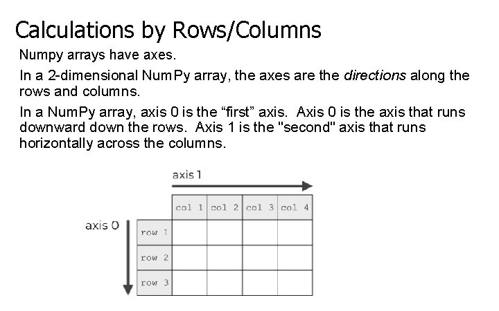
Calculations by Rows/Columns Numpy arrays have axes. In a 2 -dimensional Num. Py array, the axes are the directions along the rows and columns. In a Num. Py array, axis 0 is the “first” axis. Axis 0 is the axis that runs downward down the rows. Axis 1 is the "second" axis that runs horizontally across the columns.

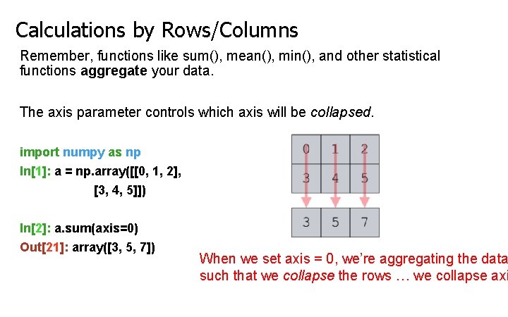
Calculations by Rows/Columns Remember, functions like sum(), mean(), min(), and other statistical functions aggregate your data. The axis parameter controls which axis will be collapsed. import numpy as np In[1]: a = np. array([[0, 1, 2], [3, 4, 5]]) In[2]: a. sum(axis=0) Out[21]: array([3, 5, 7]) When we set axis = 0, we’re aggregating the data such that we collapse the rows … we collapse axi

Calculations by Rows/Columns import numpy as np In[1]: a = np. array([[0, 1, 2], [3, 4, 5]]) In[2]: a. sum(axis=1) Out[2]: array([3, 12]) When we set axis = 1, we’re aggregating the data such that we collapse the columns … we collapse axis 1.

An Application import numpy as np Test 1 Test 2 Test 3 In[1]: grades = np. array([[87, 96, 70], Suppose we have four students, each took thre [100, 87, 90], tests. Their scores are stored [94, 77, 90], in the grades array. [100, 81, 82]]) In[3]: grades. mean(axis=0) What does this compute? Out[2]: array([95. 25, 83. ]) The average of each test. In[3]: grades. mean(axis=1) Out[2]: What does this compute? The average of each 87. 66666667]) student across all three tests. array([84. 3333, 92. 3333, 87. ,

References 1) Paul Deitel, Harvey Deitel. Intro to Python for Computer Science and Data Science, Pearson.