
Introduction to Probability Theory Rong Jin Outline o

Introduction to Probability Theory Rong Jin
Outline o o o Basic concepts in probability theory Bayes’ rule Random variable and distributions
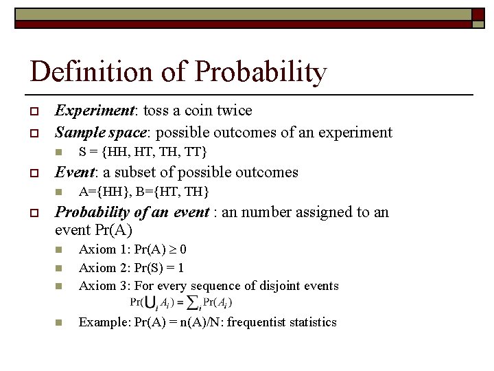
Definition of Probability o o Experiment: toss a coin twice Sample space: possible outcomes of an experiment n o Event: a subset of possible outcomes n o S = {HH, HT, TH, TT} A={HH}, B={HT, TH} Probability of an event : an number assigned to an event Pr(A) n Axiom 1: Pr(A) 0 Axiom 2: Pr(S) = 1 Axiom 3: For every sequence of disjoint events n Example: Pr(A) = n(A)/N: frequentist statistics n n
Joint Probability o For events A and B, joint probability Pr(AB) stands for the probability that both events happen. o Example: A={HH}, B={HT, TH}, what is the joint probability Pr(AB)?
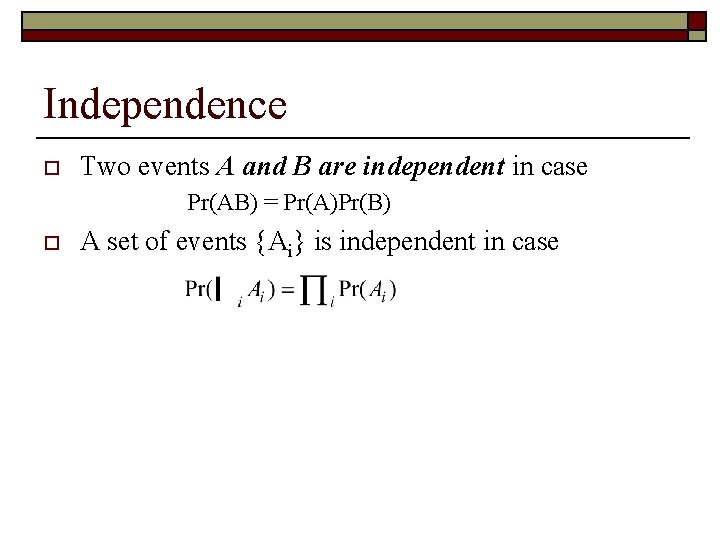
Independence o Two events A and B are independent in case Pr(AB) = Pr(A)Pr(B) o A set of events {Ai} is independent in case
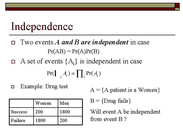
Independence o Two events A and B are independent in case Pr(AB) = Pr(A)Pr(B) o A set of events {Ai} is independent in case o Example: Drug test Women Men Success 200 1800 Failure 1800 200 A = {A patient is a Women} B = {Drug fails} Will event A be independent from event B ?
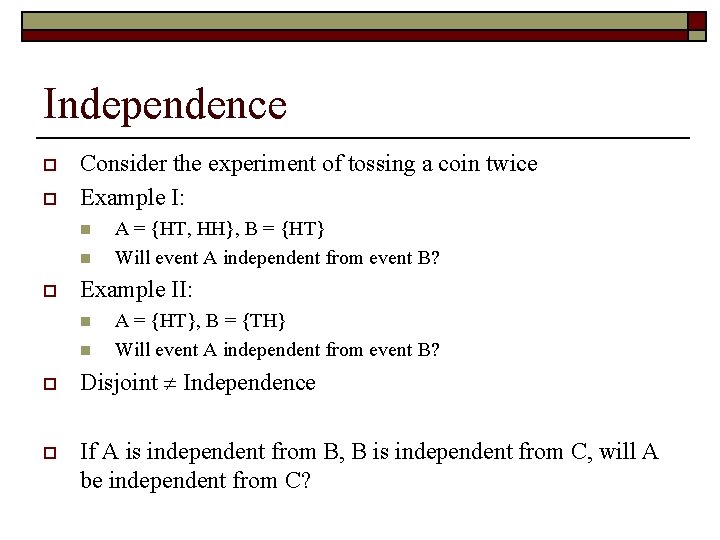
Independence o o Consider the experiment of tossing a coin twice Example I: n n o A = {HT, HH}, B = {HT} Will event A independent from event B? Example II: n n A = {HT}, B = {TH} Will event A independent from event B? o Disjoint Independence o If A is independent from B, B is independent from C, will A be independent from C?
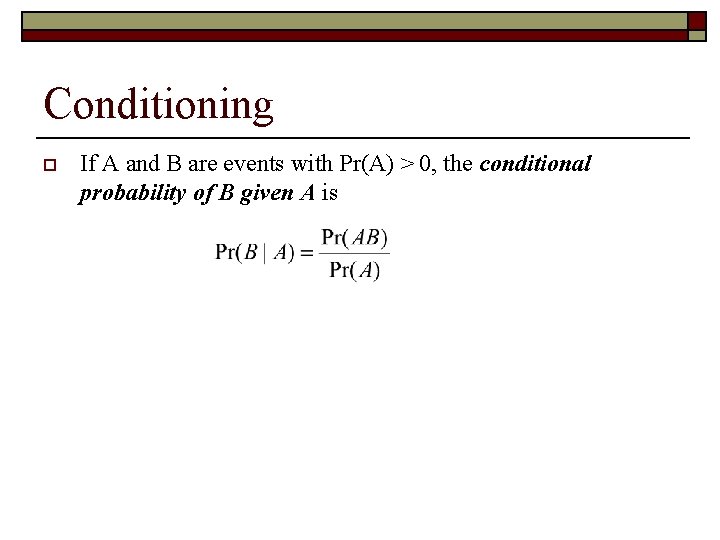
Conditioning o If A and B are events with Pr(A) > 0, the conditional probability of B given A is
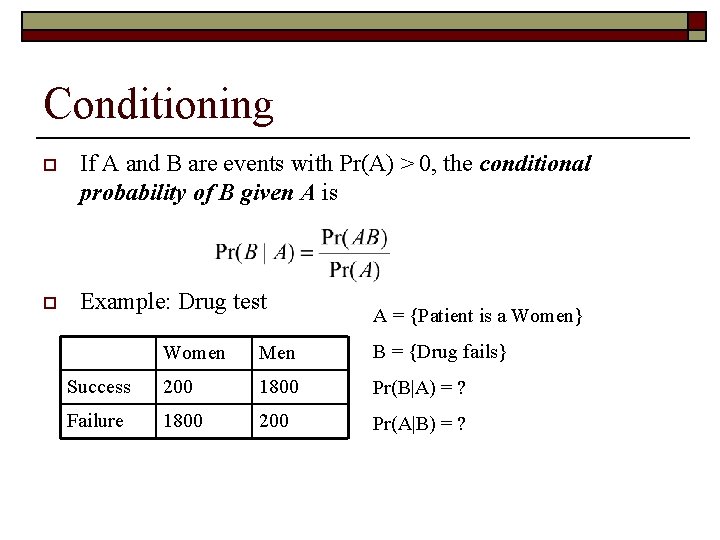
Conditioning o If A and B are events with Pr(A) > 0, the conditional probability of B given A is o Example: Drug test A = {Patient is a Women} Women Men B = {Drug fails} Success 200 1800 Pr(B|A) = ? Failure 1800 200 Pr(A|B) = ?
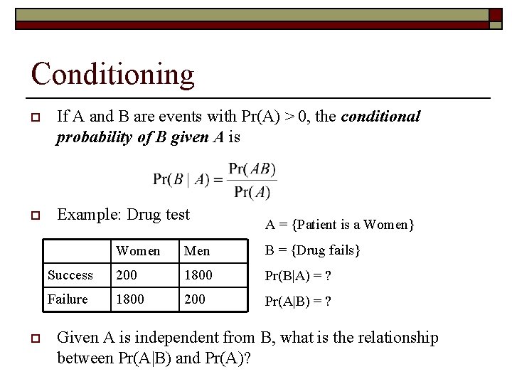
Conditioning o If A and B are events with Pr(A) > 0, the conditional probability of B given A is o Example: Drug test o A = {Patient is a Women} Women Men B = {Drug fails} Success 200 1800 Pr(B|A) = ? Failure 1800 200 Pr(A|B) = ? Given A is independent from B, what is the relationship between Pr(A|B) and Pr(A)?
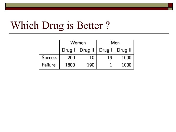
Which Drug is Better ?
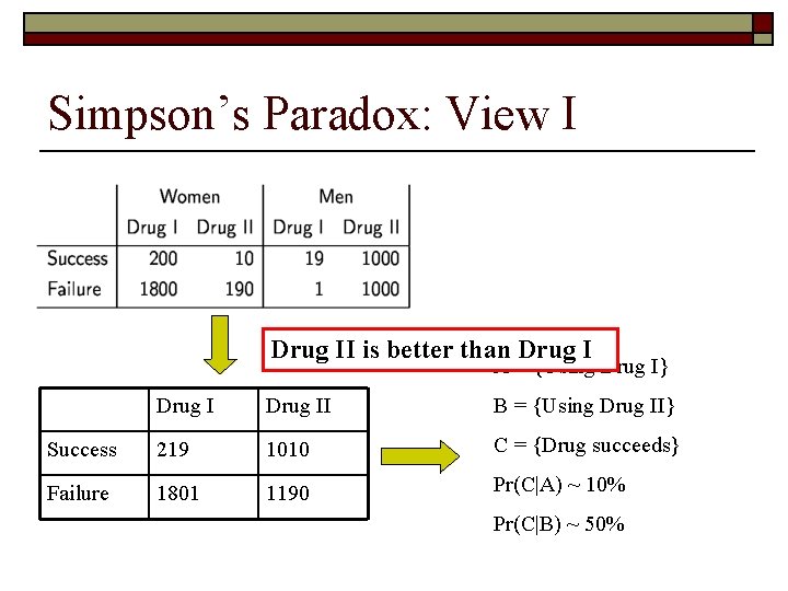
Simpson’s Paradox: View I Drug II is better than Drug I A = {Using Drug I} Drug II B = {Using Drug II} Success 219 1010 C = {Drug succeeds} Failure 1801 1190 Pr(C|A) ~ 10% Pr(C|B) ~ 50%
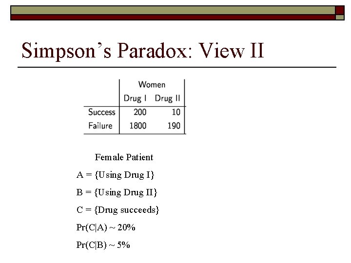
Simpson’s Paradox: View II Female Patient A = {Using Drug I} B = {Using Drug II} C = {Drug succeeds} Pr(C|A) ~ 20% Pr(C|B) ~ 5%
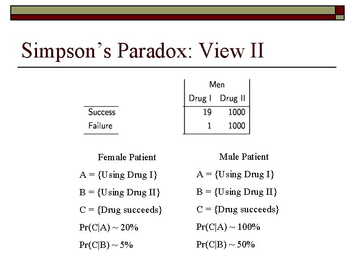
Simpson’s Paradox: View II Female Patient Male Patient A = {Using Drug I} B = {Using Drug II} C = {Drug succeeds} Pr(C|A) ~ 20% Pr(C|A) ~ 100% Pr(C|B) ~ 50%
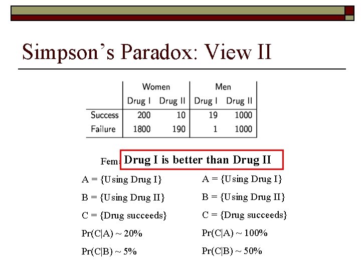
Simpson’s Paradox: View II Drug I is Female Patient better than. Male Drug II Patient A = {Using Drug I} B = {Using Drug II} C = {Drug succeeds} Pr(C|A) ~ 20% Pr(C|A) ~ 100% Pr(C|B) ~ 50%

Conditional Independence o o Event A and B are conditionally independent given C in case Pr(AB|C)=Pr(A|C)Pr(B|C) A set of events {Ai} is conditionally independent given C in case
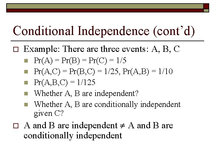
Conditional Independence (cont’d) o Example: There are three events: A, B, C n n n o Pr(A) = Pr(B) = Pr(C) = 1/5 Pr(A, C) = Pr(B, C) = 1/25, Pr(A, B) = 1/10 Pr(A, B, C) = 1/125 Whether A, B are independent? Whether A, B are conditionally independent given C? A and B are independent A and B are conditionally independent
Outline o o o Important concepts in probability theory Bayes’ rule Random variables and distributions
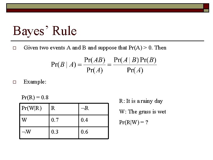
Bayes’ Rule o Given two events A and B and suppose that Pr(A) > 0. Then o Example: Pr(R) = 0. 8 Pr(W|R) R R W 0. 7 0. 4 W 0. 3 0. 6 R: It is a rainy day W: The grass is wet Pr(R|W) = ?
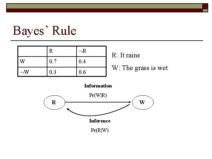
Bayes’ Rule R R W 0. 7 0. 4 W 0. 3 0. 6 R: It rains W: The grass is wet Information Pr(W|R) R W Inference Pr(R|W)
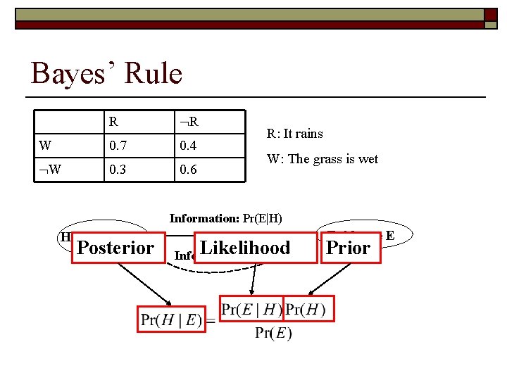
Bayes’ Rule R R W 0. 7 0. 4 W 0. 3 0. 6 R: It rains W: The grass is wet Information: Pr(E|H) Hypothesis H Posterior Likelihood Inference: Pr(H|E) Evidence E Prior
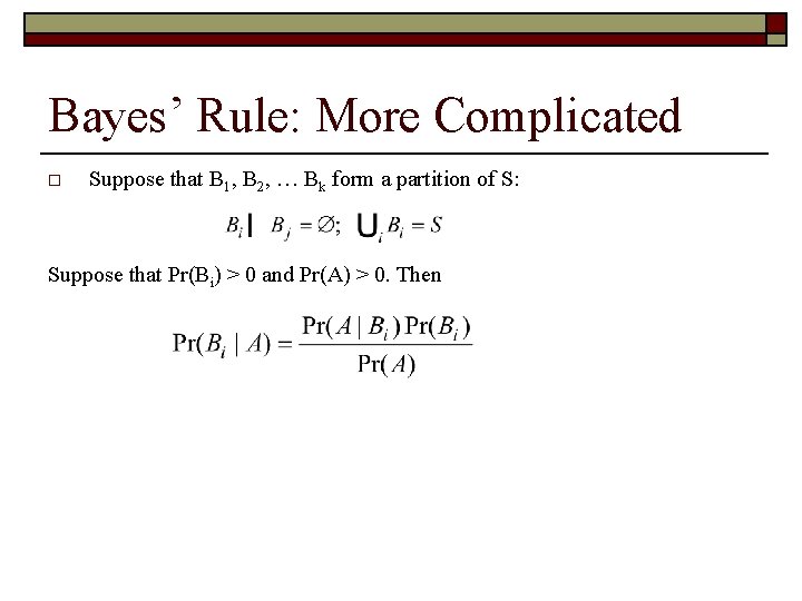
Bayes’ Rule: More Complicated o Suppose that B 1, B 2, … Bk form a partition of S: Suppose that Pr(Bi) > 0 and Pr(A) > 0. Then
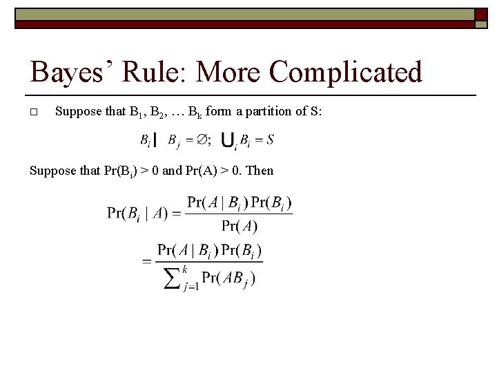
Bayes’ Rule: More Complicated o Suppose that B 1, B 2, … Bk form a partition of S: Suppose that Pr(Bi) > 0 and Pr(A) > 0. Then
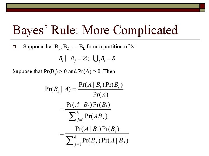
Bayes’ Rule: More Complicated o Suppose that B 1, B 2, … Bk form a partition of S: Suppose that Pr(Bi) > 0 and Pr(A) > 0. Then

A More Complicated Example R W U R It rains W The grass is wet U People bring umbrella Pr(UW|R)=Pr(U|R)Pr(W|R) Pr(UW| R)=Pr(U| R)Pr(W| R) Pr(R) = 0. 8 Pr(W|R) R R Pr(U|R) R R W 0. 7 0. 4 U 0. 9 0. 2 W 0. 3 0. 6 U 0. 1 0. 8 Pr(U|W) = ?
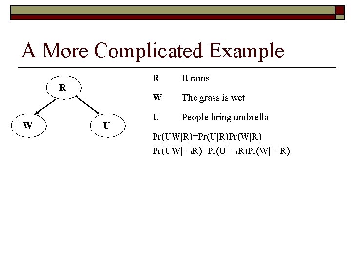
A More Complicated Example R W U R It rains W The grass is wet U People bring umbrella Pr(UW|R)=Pr(U|R)Pr(W|R) Pr(UW| R)=Pr(U| R)Pr(W| R) Pr(R) = 0. 8 Pr(W|R) R R Pr(U|R) R R W 0. 7 0. 4 U 0. 9 0. 2 W 0. 3 0. 6 U 0. 1 0. 8 Pr(U|W) = ?
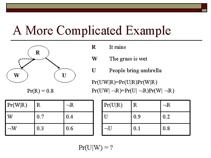
A More Complicated Example R W U R It rains W The grass is wet U People bring umbrella Pr(UW|R)=Pr(U|R)Pr(W|R) Pr(UW| R)=Pr(U| R)Pr(W| R) Pr(R) = 0. 8 Pr(W|R) R R Pr(U|R) R R W 0. 7 0. 4 U 0. 9 0. 2 W 0. 3 0. 6 U 0. 1 0. 8 Pr(U|W) = ?
Outline o o o Important concepts in probability theory Bayes’ rule Random variable and probability distribution
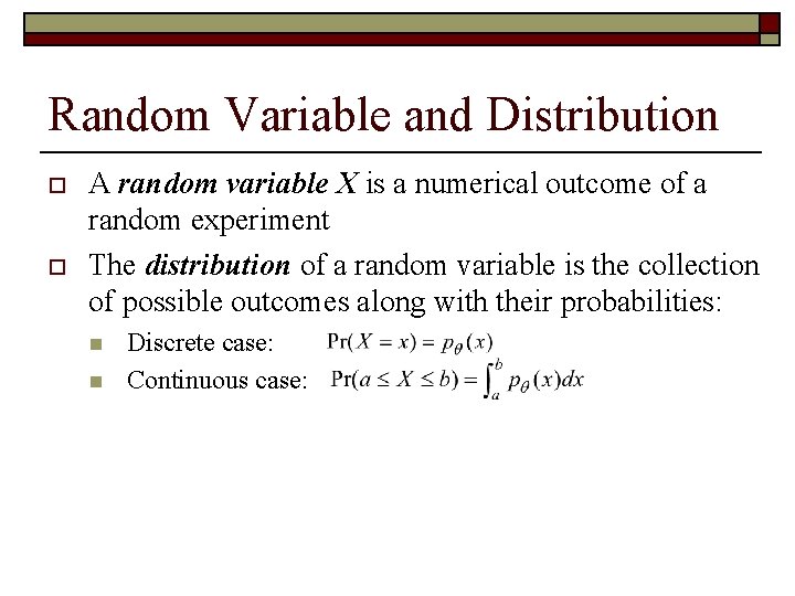
Random Variable and Distribution o o A random variable X is a numerical outcome of a random experiment The distribution of a random variable is the collection of possible outcomes along with their probabilities: n n Discrete case: Continuous case:
Random Variable: Example o o o Let S be the set of all sequences of three rolls of a die. Let X be the sum of the number of dots on the three rolls. What are the possible values for X? Pr(X = 5) = ? , Pr(X = 10) = ?
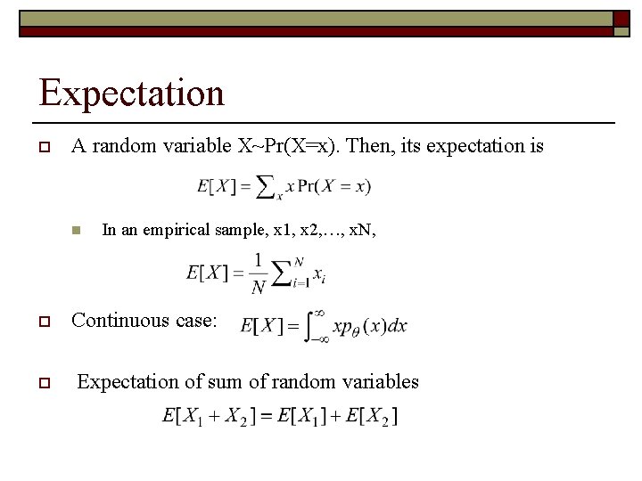
Expectation o A random variable X~Pr(X=x). Then, its expectation is n o o In an empirical sample, x 1, x 2, …, x. N, Continuous case: Expectation of sum of random variables
Expectation: Example o o Let S be the set of all sequence of three rolls of a die. Let X be the sum of the number of dots on the three rolls. What is E(X)? Let S be the set of all sequence of three rolls of a die. Let X be the product of the number of dots on the three rolls. What is E(X)?
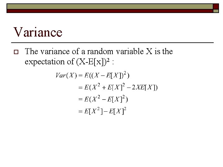
Variance o The variance of a random variable X is the expectation of (X-E[x])2 :
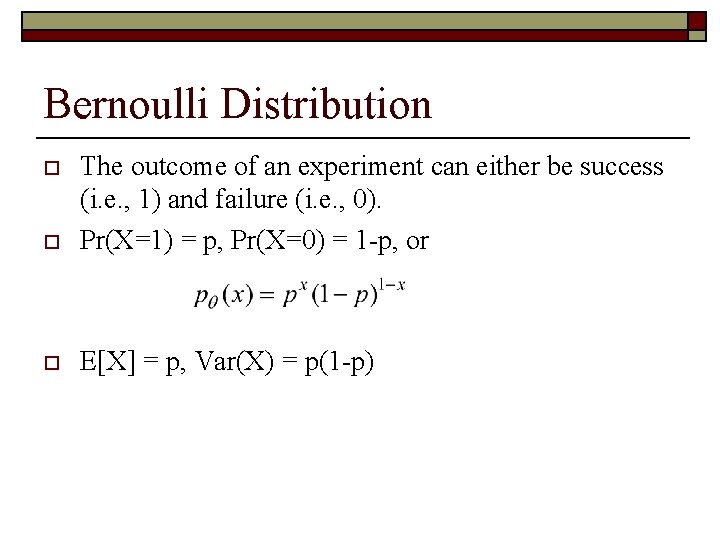
Bernoulli Distribution o The outcome of an experiment can either be success (i. e. , 1) and failure (i. e. , 0). Pr(X=1) = p, Pr(X=0) = 1 -p, or o E[X] = p, Var(X) = p(1 -p) o
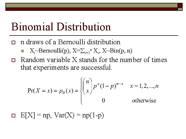
Binomial Distribution o n draws of a Bernoulli distribution n Xi~Bernoulli(p), X= i=1 n Xi, X~Bin(p, n) o Random variable X stands for the number of times that experiments are successful. o E[X] = np, Var(X) = np(1 -p)
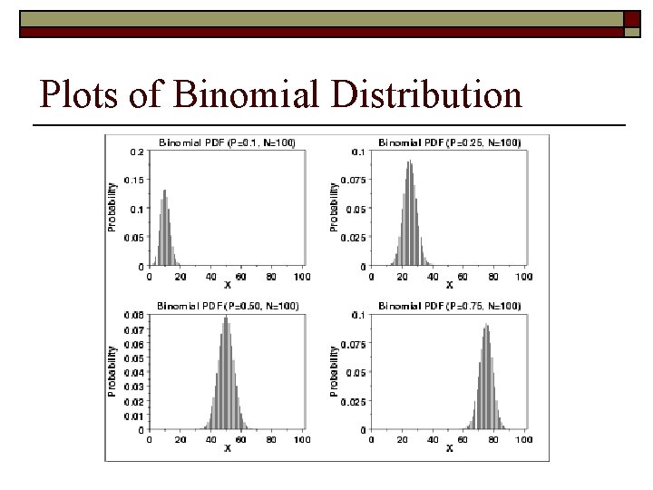
Plots of Binomial Distribution
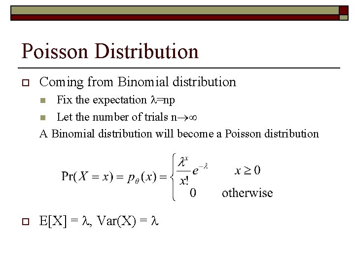
Poisson Distribution o Coming from Binomial distribution Fix the expectation =np n Let the number of trials n A Binomial distribution will become a Poisson distribution n o E[X] = , Var(X) =
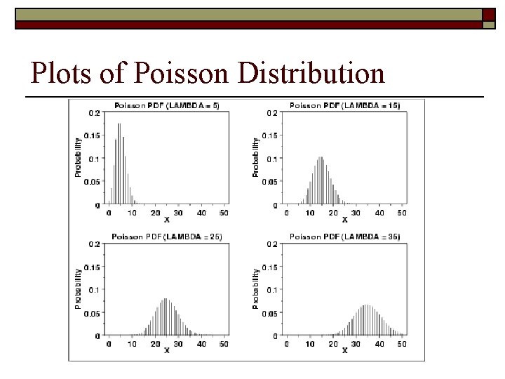
Plots of Poisson Distribution
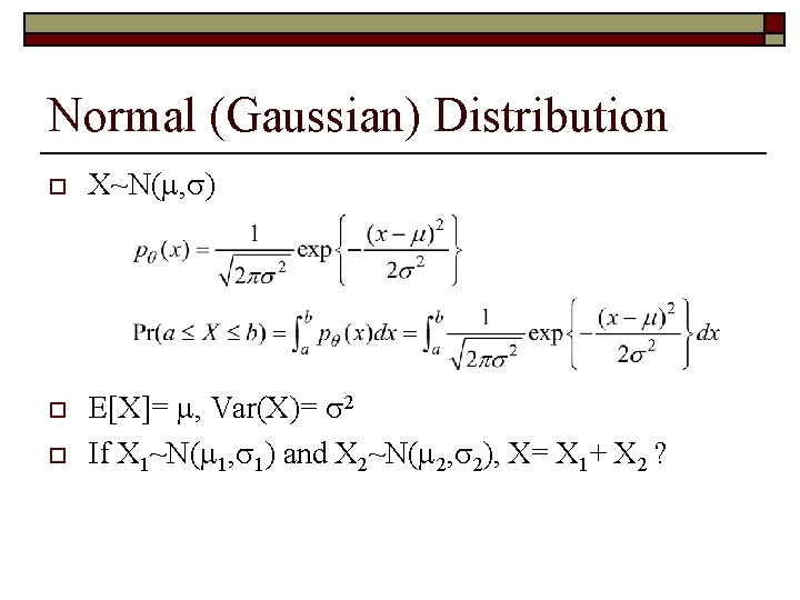
Normal (Gaussian) Distribution o o o X~N( , ) E[X]= , Var(X)= 2 If X 1~N( 1, 1) and X 2~N( 2, 2), X= X 1+ X 2 ?
- Slides: 39