Introduction to Open Mx Sarah Medland What is

Introduction to Open. Mx Sarah Medland

What is Open. Mx? • Free, Open-source, full–featured SEM package • Software which runs on Windows, Mac OSX, and Linux • A package in the R statistical programing environment • Two main approaches to writing Open. Mx models – Path or Matrix Specification

• R is a functional language • Easy to define new functions • Items are stored as Objects • Open. Mx uses functions to build objects • Arguments to the function have an order • Order can be changed by naming arguments

Matrices are the building blocks Matrix: a rectangular array of elements arranged in rows and columns. The order or dimension of a matrix is defined by the number of row and columns in the matrix. Columns (3 x 3) d g b e h c f i Rows A = a The order of a matrix is generally referred to as M x N (where M is the number of rows and N is the number of columns) Matrix A is a 3 x 3 matrix. Each element in the matrix is referred to by its placement in a row and column, where aij is the element in Matrix A in the ith row and jth column. Therefore, e is element a(2, 2)

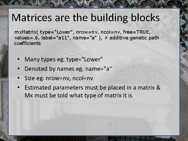
Matrices are the building blocks mx. Matrix( type="Lower", nrow=nv, ncol=nv, free=TRUE, values=. 6, label="a 11", name="a" ), # additive genetic path coefficients • • Many types eg. type="Lower" Denoted by names eg. name="a“ Size eg. nrow=nv, ncol=nv Estimated parameters must be placed in a matrix & Mx must be told what type of matrix it is

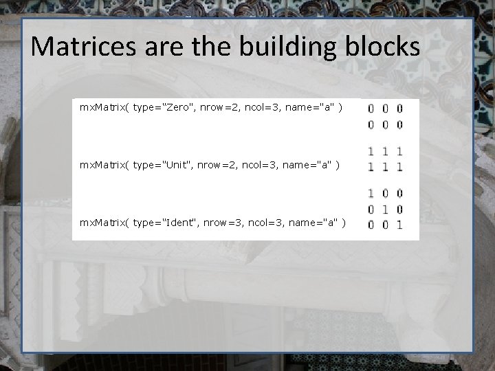
Matrices are the building blocks mx. Matrix( type=“Zero", nrow=2, ncol=3, name="a" ) mx. Matrix( type=“Unit", nrow=2, ncol=3, name="a" ) mx. Matrix( type=“Ident", nrow=3, ncol=3, name="a" )

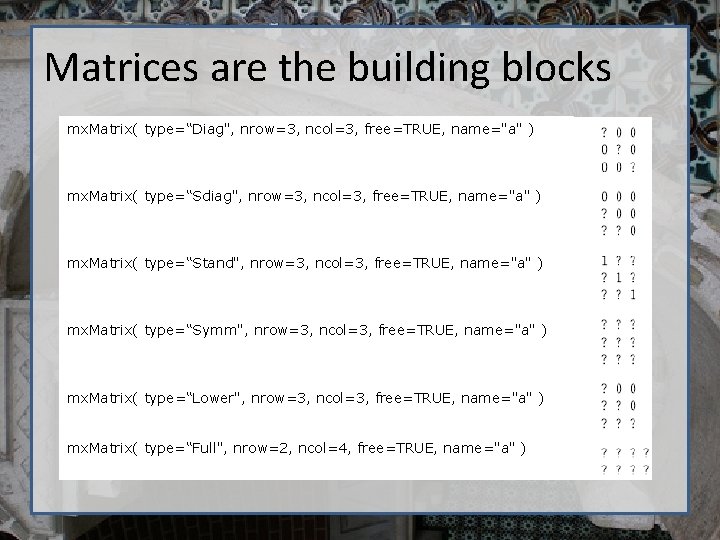
Matrices are the building blocks mx. Matrix( type=“Diag", nrow=3, ncol=3, free=TRUE, name="a" ) • Many types mx. Matrix( type=“Sdiag", nrow=3, ncol=3, free=TRUE, name="a" ) mx. Matrix( type=“Stand", nrow=3, ncol=3, free=TRUE, name="a" ) mx. Matrix( type=“Symm", nrow=3, ncol=3, free=TRUE, name="a" ) mx. Matrix( type=“Lower", nrow=3, ncol=3, free=TRUE, name="a" ) mx. Matrix( type=“Full", nrow=2, ncol=4, free=TRUE, name="a" )

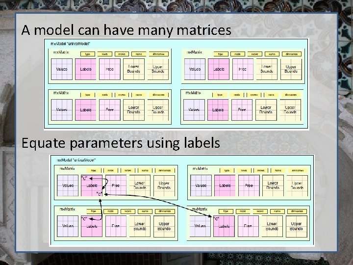
A model can have many matrices Equate parameters using labels

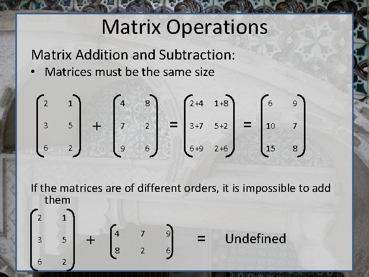
Matrix Operations Matrix Addition and Subtraction: • Matrices must be the same size 2 1 3 5 6 2 + 4 8 7 2 9 6 = 2+4 1+8 3+7 5+2 6+9 2+6 = 6 9 10 7 15 8 If the matrices are of different orders, it is impossible to add them 2 1 3 5 6 2 + 4 7 9 8 2 6 = Undefined

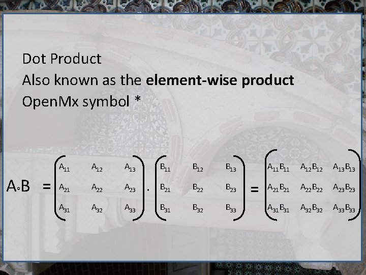
Dot Product Also known as the element-wise product Open. Mx symbol * AB = A 11 A 12 A 13 A 21 A 22 A 23 A 31 A 32 A 33 B 11 B 12 B 13 B 21 B 22 B 23 B 31 B 32 B 33 = A 11 B 11 A 12 B 12 A 13 B 13 A 21 B 21 A 22 B 22 A 23 B 23 A 31 B 31 A 32 B 32 A 33 B 33

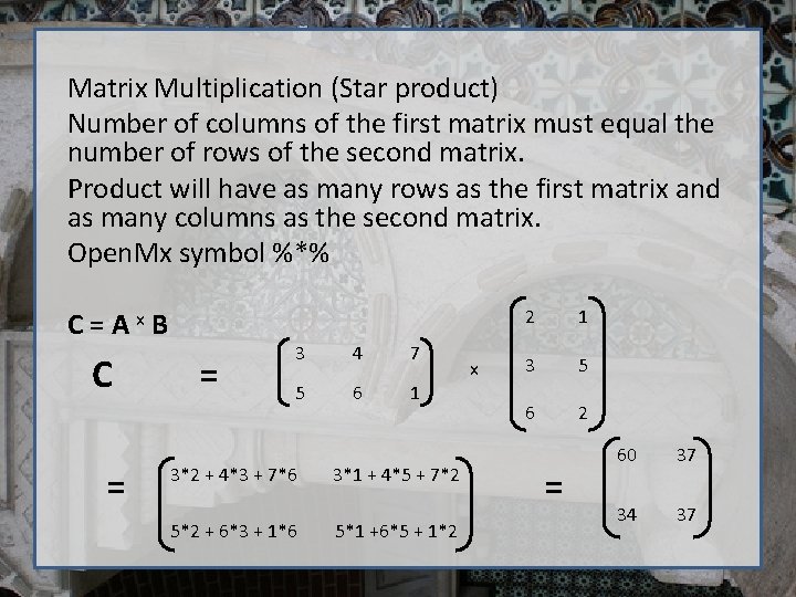
Matrix Multiplication (Star product) Number of columns of the first matrix must equal the number of rows of the second matrix. Product will have as many rows as the first matrix and as many columns as the second matrix. Open. Mx symbol %*% C=Ax. B C = = 3 4 7 5 6 1 3*2 + 4*3 + 7*6 5*2 + 6*3 + 1*6 3*1 + 4*5 + 7*2 5*1 +6*5 + 1*2 x 2 1 3 5 6 2 = 60 37 34 37

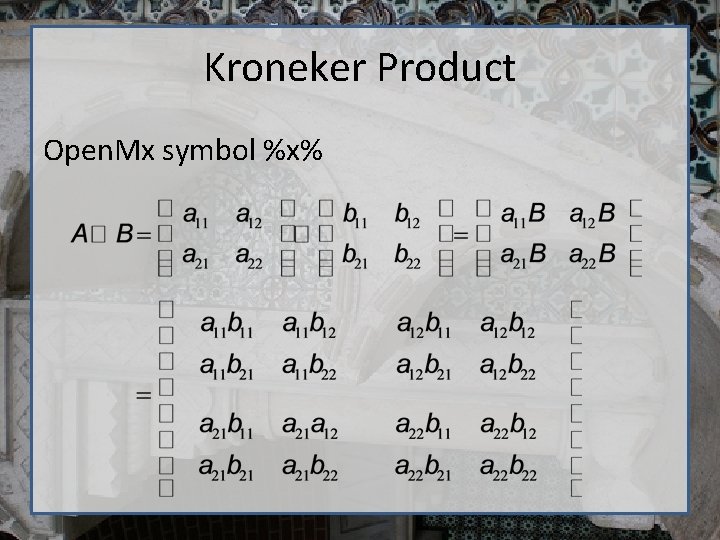
Kroneker Product Open. Mx symbol %x%

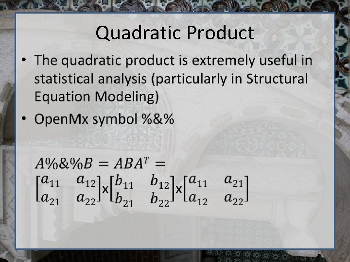
Quadratic Product •

Our first Open. Mx script • Linear regression ( aka simple regression, Ordinary Least Squares Regression, linear model) • Raw data • Describe the relationship between two variables, X and Y, as a straight line • The regression of BMI on variable Age – Does age predict BMI? BMI=weight in kg/ (height in m)2

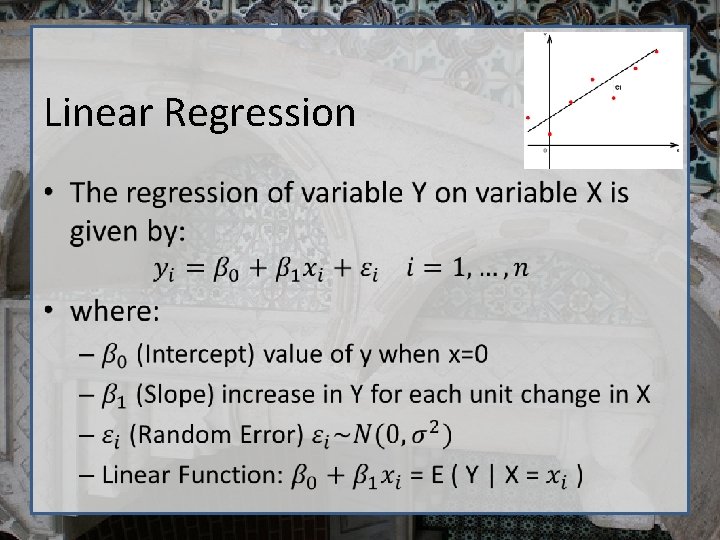
Linear Regression •

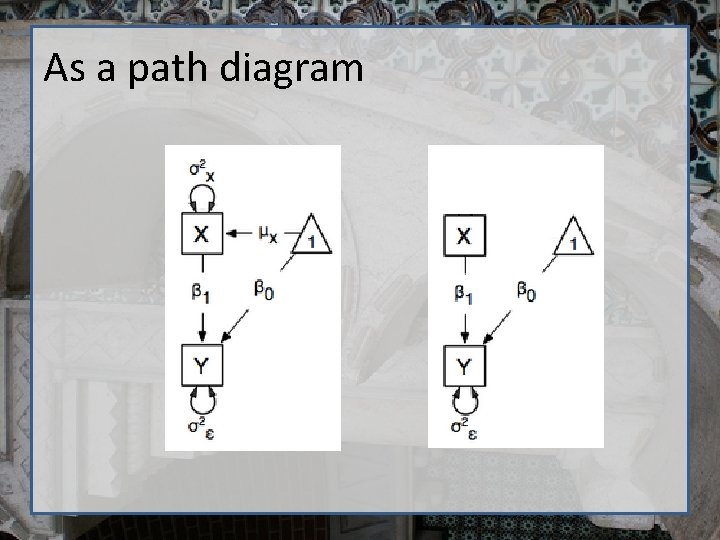
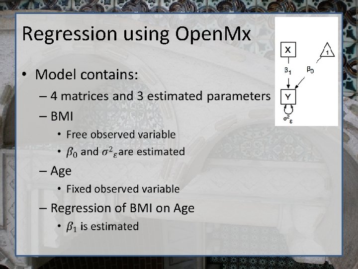
As a path diagram

Starting at the beginning… • Data preparation – The algebra style used in Open. Mx expects 1 line per case/family – (Almost) limitless number of families and variables – Data needs to be read into R before it can be analysed • (the commands to read the data can be nested within the R script) • Default missing code is now NA

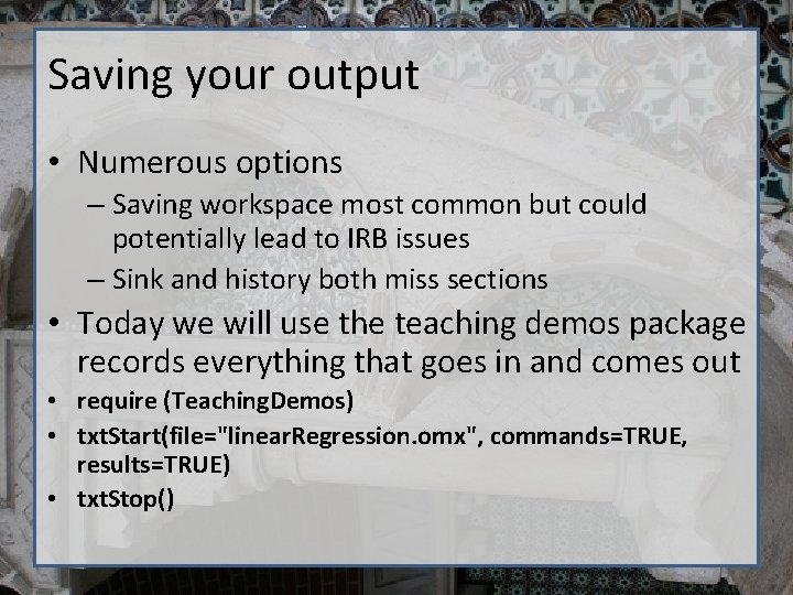
Saving your output • Numerous options – Saving workspace most common but could potentially lead to IRB issues – Sink and history both miss sections • Today we will use the teaching demos package records everything that goes in and comes out • require (Teaching. Demos) • txt. Start(file="linear. Regression. omx", commands=TRUE, results=TRUE) • txt. Stop()

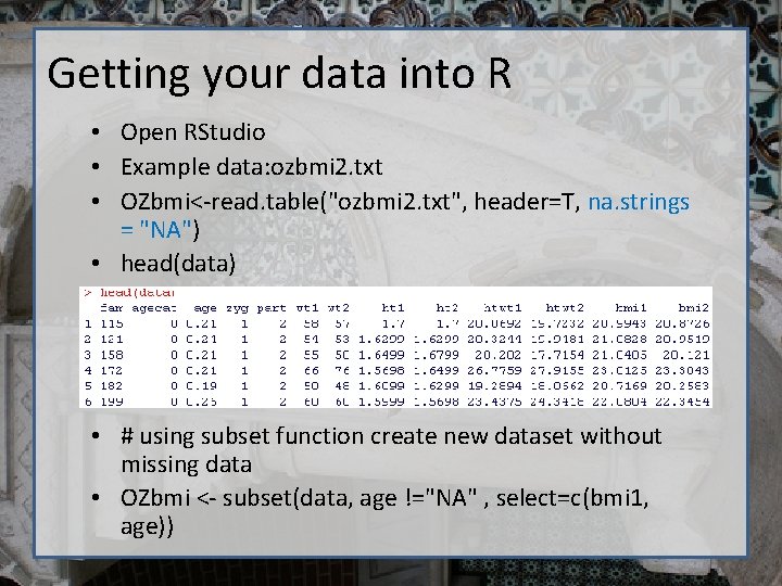
Getting your data into R • Open RStudio • Example data: ozbmi 2. txt • OZbmi<-read. table("ozbmi 2. txt", header=T, na. strings = "NA") • head(data) • # using subset function create new dataset without missing data • OZbmi <- subset(data, age !="NA" , select=c(bmi 1, age))

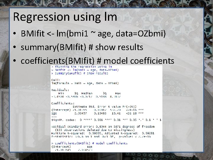
Regression using lm • BMIfit <- lm(bmi 1 ~ age, data=OZbmi) • summary(BMIfit) # show results • coefficients(BMIfit) # model coefficients

Regression using Open. Mx •

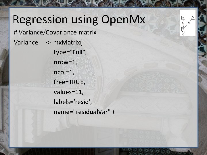
Regression using Open. Mx # Variance/Covariance matrix Variance <- mx. Matrix( type="Full", nrow=1, ncol=1, free=TRUE, values=11, labels='resid', name="residual. Var" )

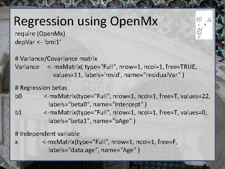
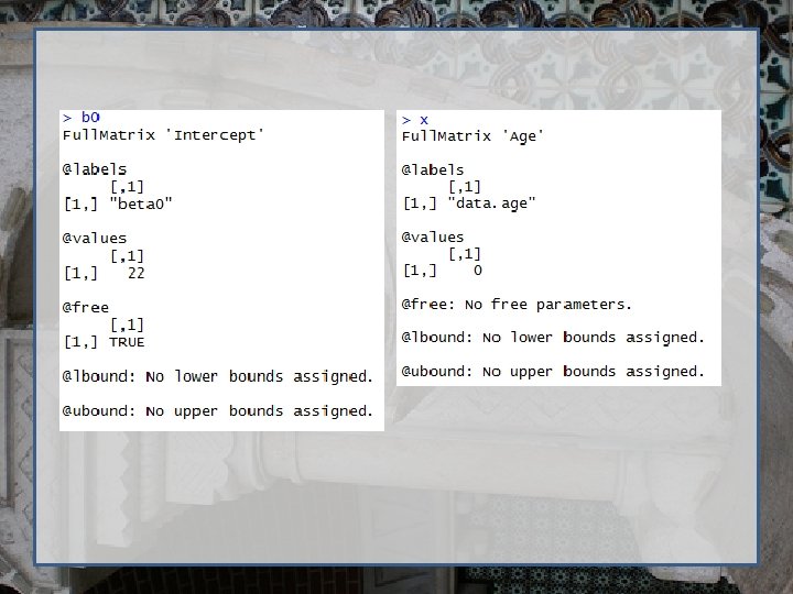
Regression using Open. Mx require (Open. Mx) dep. Var <- 'bmi 1‘ # Variance/Covariance matrix Variance <- mx. Matrix( type="Full", nrow=1, ncol=1, free=TRUE, values=11, labels='resid', name="residual. Var" ) # Regression betas b 0 <-mx. Matrix(type="Full", nrow=1, ncol=1, free=T, values=22, labels="beta 0", name="Intercept" ) b 1 <-mx. Matrix(type="Full", nrow=1, ncol=1, free=T, values=0, labels="beta 1", name="b. Age" ) # Independent variable x <-mx. Matrix(type="Full", nrow=1, ncol=1, free=F, labels="data. age", name="Age" )

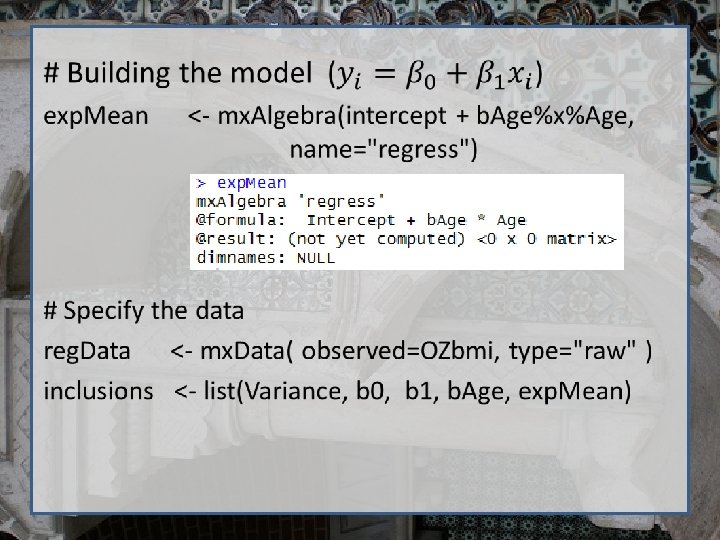
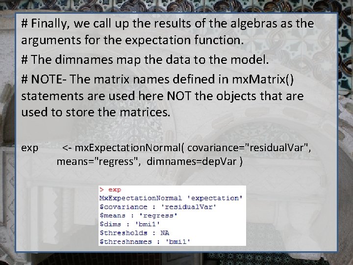
# Finally, we call up the results of the algebras as the arguments for the expectation function. # The dimnames map the data to the model. # NOTE- The matrix names defined in mx. Matrix() statements are used here NOT the objects that are used to store the matrices. exp <- mx. Expectation. Normal( covariance="residual. Var", means="regress", dimnames=dep. Var )

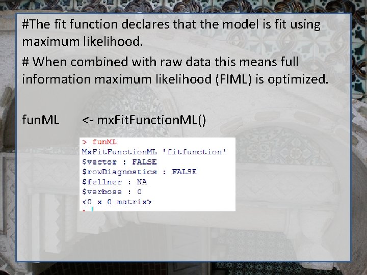
#The fit function declares that the model is fit using maximum likelihood. # When combined with raw data this means full information maximum likelihood (FIML) is optimized. fun. ML <- mx. Fit. Function. ML()

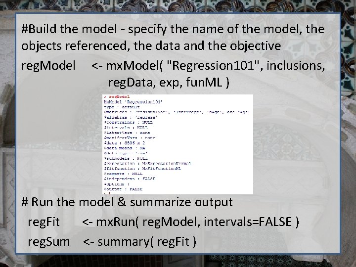
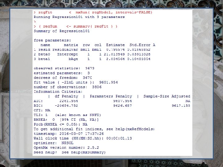
#Build the model - specify the name of the model, the objects referenced, the data and the objective reg. Model <- mx. Model( "Regression 101", inclusions, reg. Data, exp, fun. ML ) # Run the model & summarize output reg. Fit <- mx. Run( reg. Model, intervals=FALSE ) reg. Sum <- summary( reg. Fit )

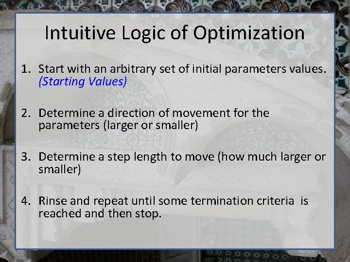
Intuitive Logic of Optimization 1. Start with an arbitrary set of initial parameters values. (Starting Values) 2. Determine a direction of movement for the parameters (larger or smaller) 3. Determine a step length to move (how much larger or smaller) 4. Rinse and repeat until some termination criteria is reached and then stop.

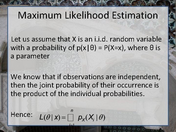
Maximum Likelihood Estimation Let us assume that X is an i. i. d. random variable with a probability of p(x|θ) = P(X=x), where θ is a parameter We know that if observations are independent, then the joint probability of their occurrence is the product of the individual probabilities. Hence:

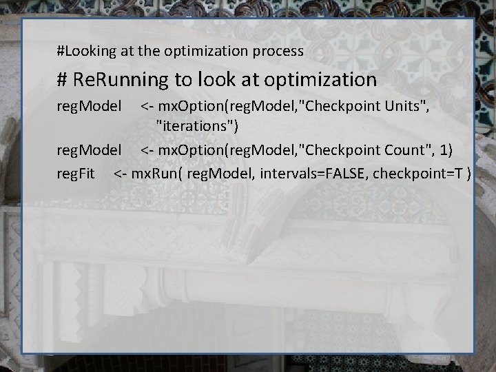
#Looking at the optimization process # Re. Running to look at optimization reg. Model <- mx. Option(reg. Model, "Checkpoint Units", "iterations") reg. Model <- mx. Option(reg. Model, "Checkpoint Count", 1) reg. Fit <- mx. Run( reg. Model, intervals=FALSE, checkpoint=T )

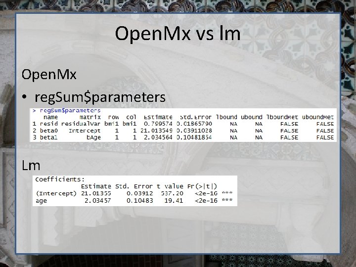
Open. Mx vs lm Open. Mx • reg. Sum$parameters Lm

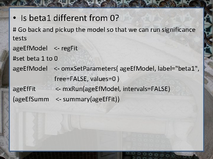
• Is beta 1 different from 0? # Go back and pickup the model so that we can run significance tests age. Ef. Model <- reg. Fit #set beta 1 to 0 age. Ef. Model <- omx. Set. Parameters( age. Ef. Model, label="beta 1", free=FALSE, values=0 ) age. Ef. Fit <- mx. Run(age. Ef. Model, intervals=FALSE) (age. Ef. Summ <- summary(age. Ef. Fit))

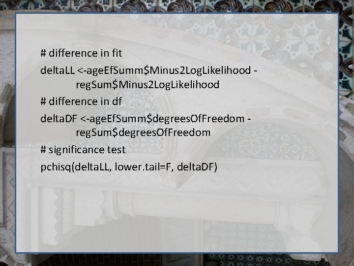
# difference in fit delta. LL <-age. Ef. Summ$Minus 2 Log. Likelihood reg. Sum$Minus 2 Log. Likelihood # difference in df delta. DF <-age. Ef. Summ$degrees. Of. Freedom reg. Sum$degrees. Of. Freedom # significance test pchisq(delta. LL, lower. tail=F, delta. DF)

Questions? Bus shelter on the road to Sintra (Portugal)