Introduction to Ocean Numerical Modeling 3 Numerical aspects

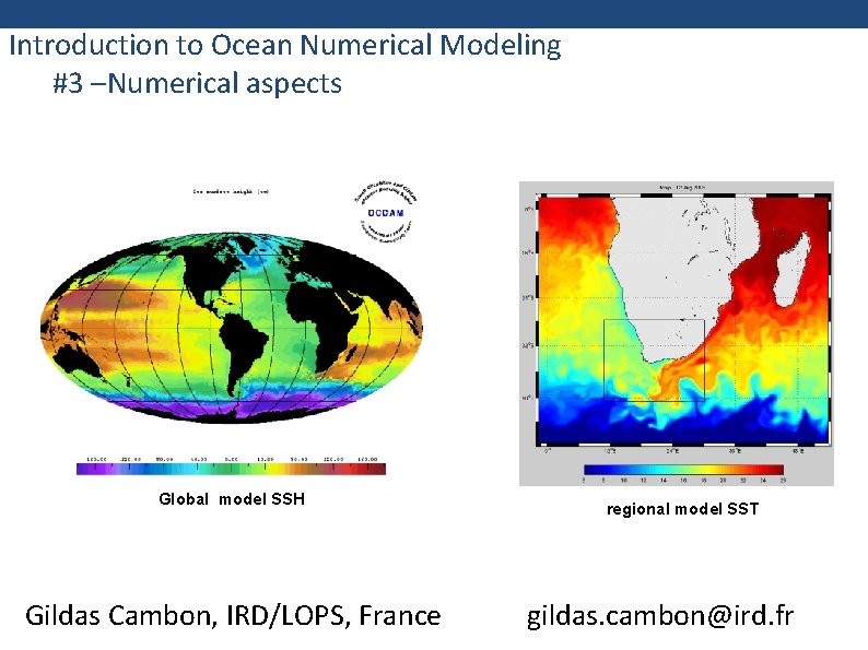
Introduction to Ocean Numerical Modeling #3 –Numerical aspects Global model SSH Gildas Cambon, IRD/LOPS, France regional model SST gildas. cambon@ird. fr

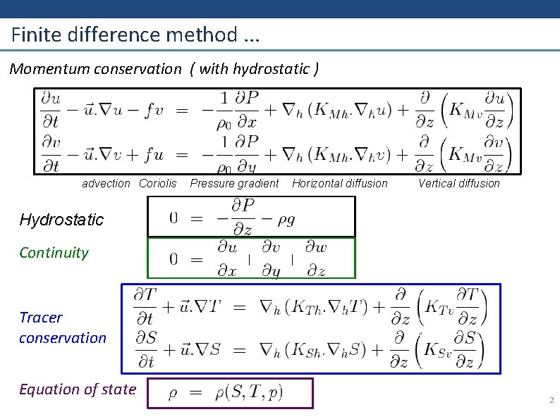
Finite difference method. . . Momentum conservation ( with hydrostatic ) advection Coriolis Pressure gradient Horizontal diffusion Vertical diffusion Hydrostatic Continuity Tracer conservation Equation of state 2

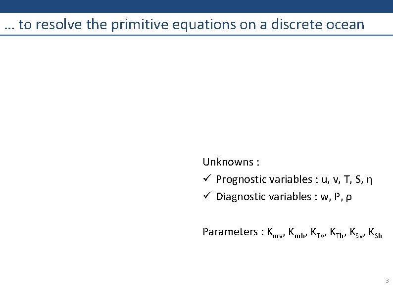
… to resolve the primitive equations on a discrete ocean Unknowns : ü Prognostic variables : u, v, T, S, η ü Diagnostic variables : w, P, ρ Parameters : Kmv, Kmh, KTv, KTh, KSv, KSh 3

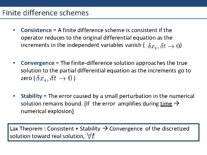
Finite difference schemes • A finite difference scheme is produced when the partial derivatives in the partial differential equations governing a physical phenomenon are replaced by a finite difference approximation. • The result is a system of algebraic equations which, when solved, provide an approximation to the solution of the original partial differential equations at selected points of a solution grid. • The Most important characteristic of a scheme are: Consistence, Stability and Convergence

Finite difference schemes • Consistence = A finite difference scheme is consistent if the operator reduces to the original differential equation as the increments in the independent variables vanish ( ) • Convergence = The finite difference solution approaches the true solution to the partial differential equation as the increments go to zero ( ) • Stability = The error caused by a small perturbation in the numerical solution remains bound. [If the error amplifies during time numerical explosion] Lax Theorem : Consistent + Stability Convergence of the discretized solution toward real solution,

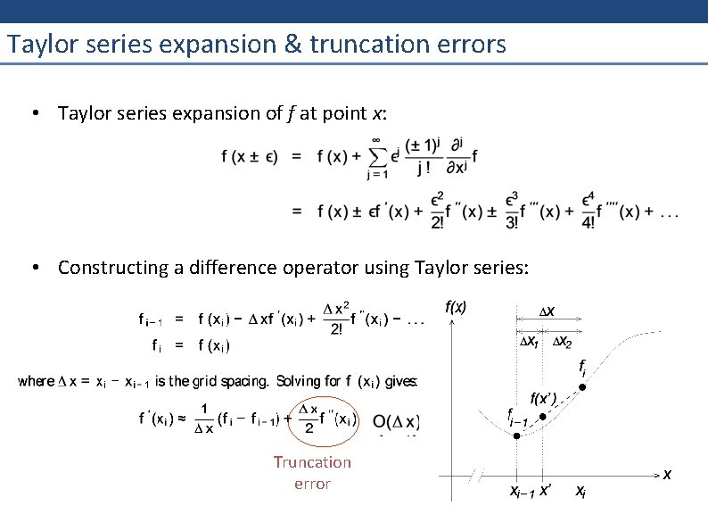
Taylor series expansion & truncation errors • Taylor series expansion of f at point x: • Constructing a difference operator using Taylor series: Truncation error

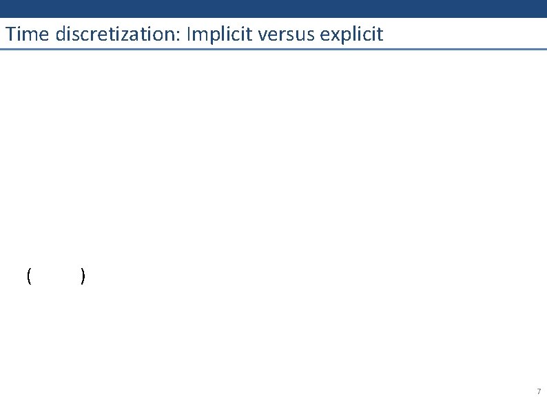
Time discretization: Implicit versus explicit ( ) 7

Time discretization: Multi levels schemes

Time discretization: Predictor– corrector and multipoint methods

Time discretization: Summary Durran, Numerical Method for Fluid Dynamics

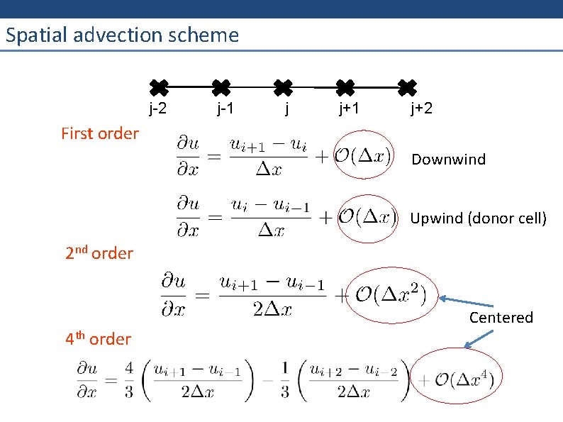
Spatial advection scheme j-2 j-1 j j+1 j+2 First order Downwind Upwind (donor cell) 2 nd order 4 th order Centered

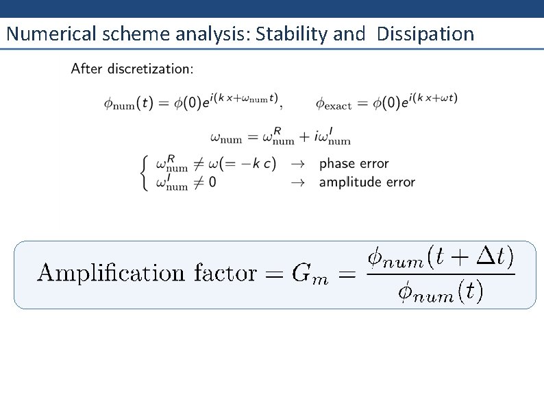
Numerical scheme analysis: Stability and Dissipation

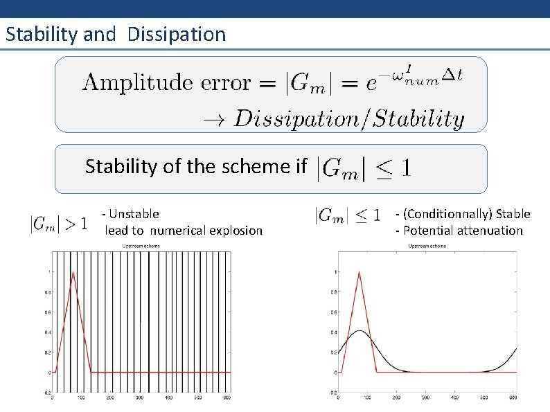
Stability and Dissipation Stability of the scheme if Unstable lead to numerical explosion (Conditionnally) Stable Potential attenuation

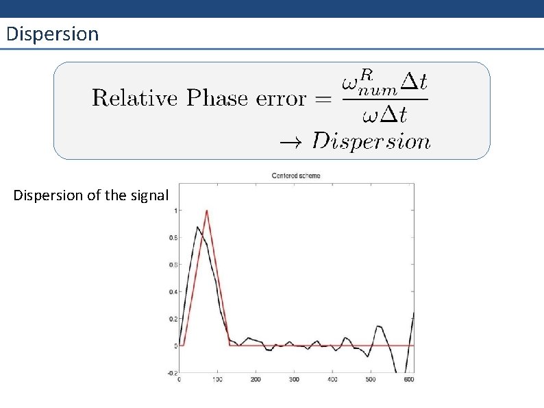
Dispersion of the signal

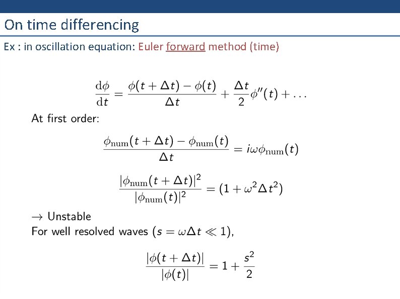
On time differencing Ex : in oscillation equation: Euler forward method (time)

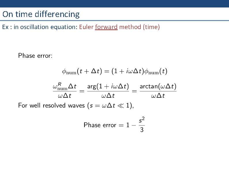
On time differencing Ex : in oscillation equation: Euler forward method (time)

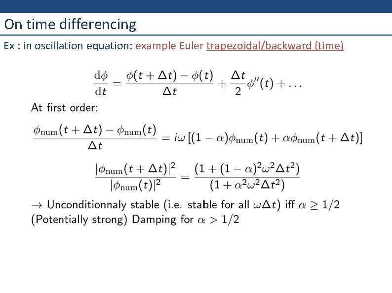
On time differencing Ex : in oscillation equation: example Euler trapezoidal/backward (time)

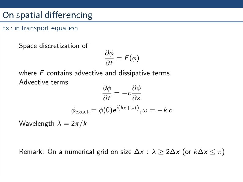
On spatial differencing Ex : in transport equation

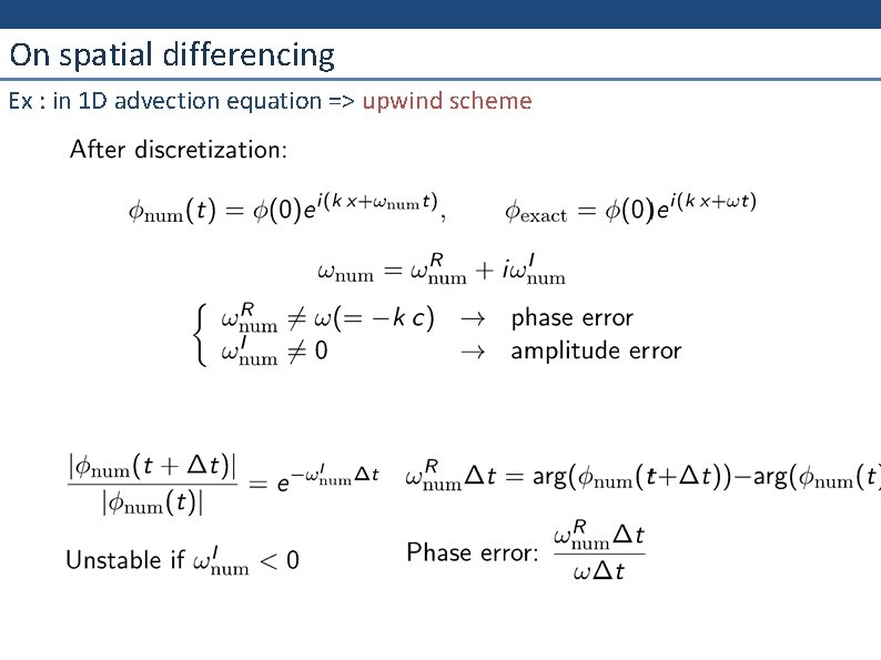
On spatial differencing Ex : in 1 D advection equation => upwind scheme

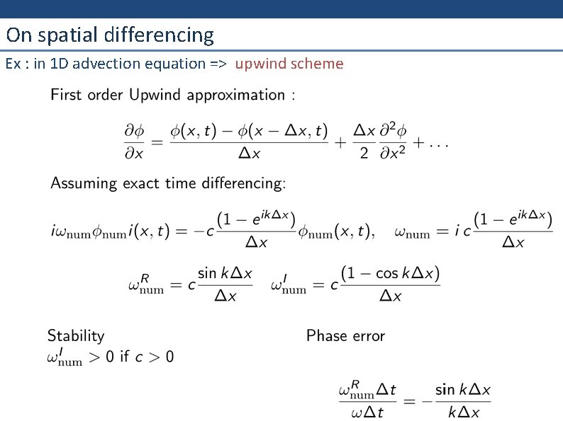
On spatial differencing Ex : in 1 D advection equation => upwind scheme

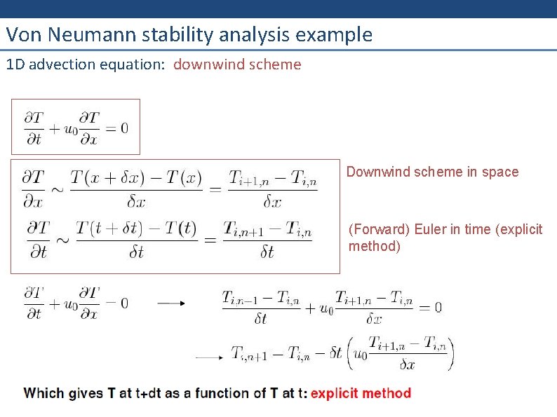
Von Neumann stability analysis example 1 D advection equation: downwind scheme Downwind scheme in space (Forward) Euler in time (explicit method)

Von Neumann stability analysis example

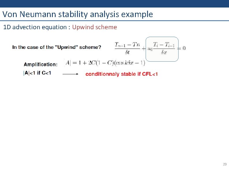
Von Neumann stability analysis example 1 D advection equation : Upwind scheme 23

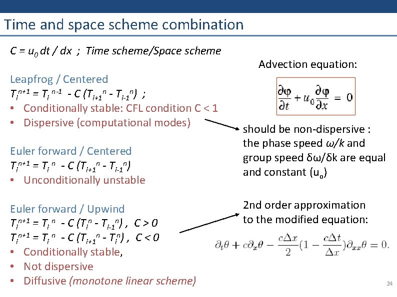
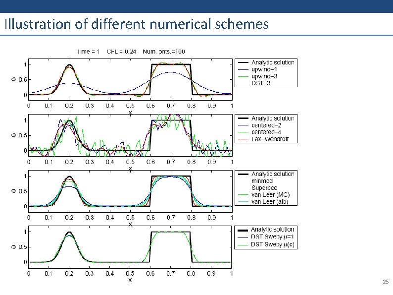
Time and space scheme combination C = u 0 dt / dx ; Time scheme/Space scheme Leapfrog / Centered Tin+1 = Ti n-1 - C (Ti+1 n - Ti-1 n) ; • Conditionally stable: CFL condition C < 1 • Dispersive (computational modes) Euler forward / Centered Tin+1 = Ti n - C (Ti+1 n - Ti-1 n) • Unconditionally unstable Euler forward / Upwind Tin+1 = Ti n - C (Tin - Ti-1 n) , C > 0 Tin+1 = Ti n - C (Ti+1 n - Tin) , C < 0 • Conditionally stable, • Not dispersive • Diffusive (monotone linear scheme) Advection equation: should be non dispersive : the phase speed ω/k and group speed δω/δk are equal and constant (uo) 2 nd order approximation to the modified equation: 24

Illustration of different numerical schemes 25

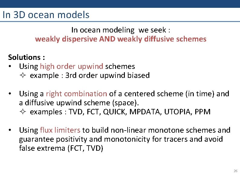
In 3 D ocean models In ocean modeling we seek : weakly dispersive AND weakly diffusive schemes Solutions : • Using high order upwind schemes ² example : 3 rd order upwind biased • Using a right combination of a centered scheme (in time) and a diffusive upwind scheme (space). ² examples : TVD, FCT, QUICK, MPDATA, UTOPIA, PPM • Using flux limiters to build non linear monotone schemes and guarantee positivity and monotonicity for tracers and avoid false extrema (FCT, TVD) 26

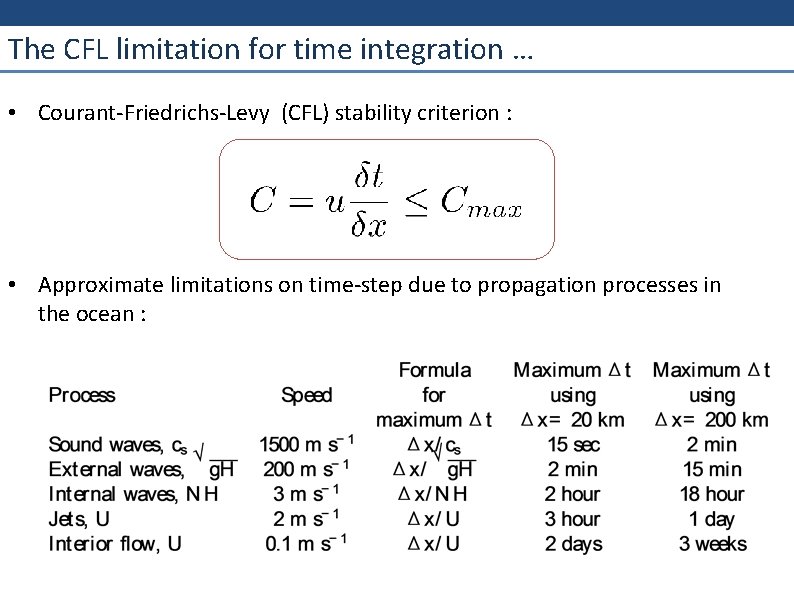
The CFL limitation for time integration … • Courant Friedrichs Levy (CFL) stability criterion : • Approximate limitations on time step due to propagation processes in the ocean :

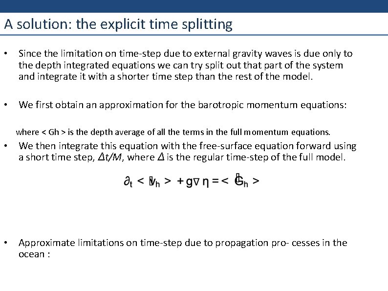
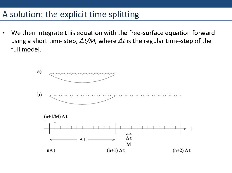
A solution: the explicit time splitting • Since the limitation on time step due to external gravity waves is due only to the depth integrated equations we can try split out that part of the system and integrate it with a shorter time step than the rest of the model. • We first obtain an approximation for the barotropic momentum equations: where < Gh > is the depth average of all the terms in the full momentum equations. • We then integrate this equation with the free surface equation forward using a short time step, Δt/M, where Δ is the regular time step of the full model. • Approximate limitations on time step due to propagation pro cesses in the ocean :

A solution: the explicit time splitting • We then integrate this equation with the free surface equation forward using a short time step, Δt/M, where Δt is the regular time step of the full model.

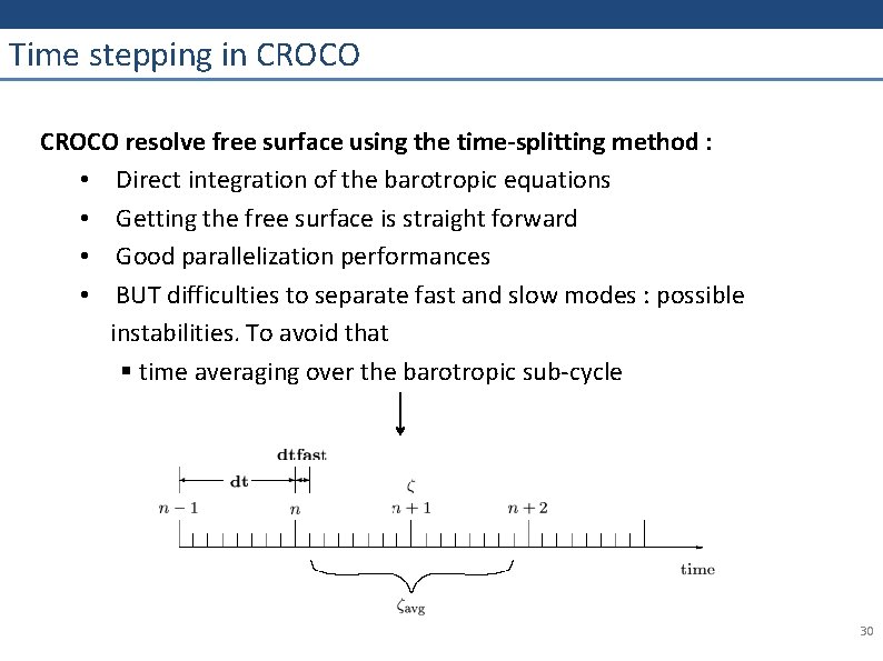
Time stepping in CROCO resolve free surface using the time-splitting method : • Direct integration of the barotropic equations • Getting the free surface is straight forward • Good parallelization performances • BUT difficulties to separate fast and slow modes : possible instabilities. To avoid that § time averaging over the barotropic sub cycle 30

Time stepping in CROCO