Introduction to Ocean Numerical Modeling 1 Equations of

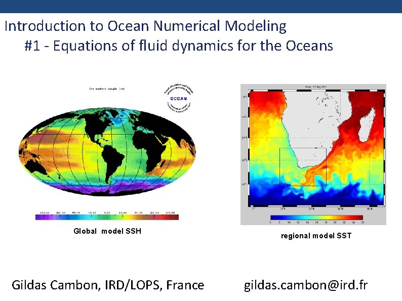
Introduction to Ocean Numerical Modeling #1 - Equations of fluid dynamics for the Oceans Global model SSH Gildas Cambon, IRD/LOPS, France regional model SST gildas. cambon@ird. fr

Outline 1. Introduction 2. Momentum conservation 3. Mass conservation 4. Heat and Salt transport 5. Equation of state 6. Full primitive equations

Introduction Ocean is a fluid 4 categories of equations 1. 2. 3. 4. Momentum conservation Mass conservation Heat and salt transport Equation of state

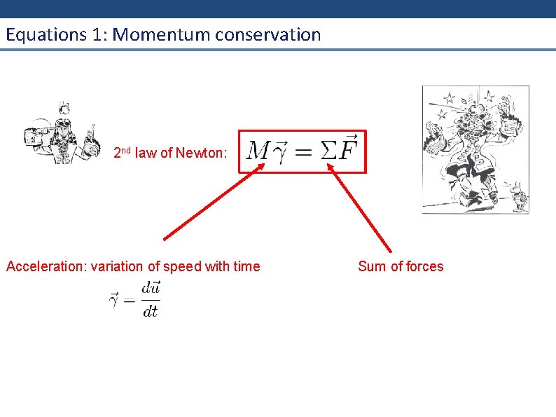
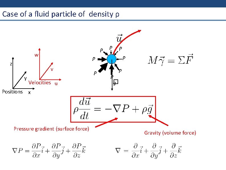
Equations 1: Momentum conservation 2 nd law of Newton: Acceleration: variation of speed with time Sum of forces

Case of a fluid particle of density ρ P w z P P P v y P Velocities u P P � g P Positions x Pressure gradient (surface force) Gravity (volume force)

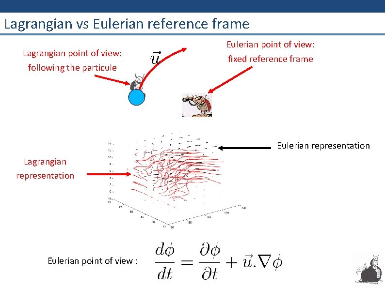
Lagrangian vs Eulerian reference frame Lagrangian point of view: following the particule Eulerian point of view: fixed reference frame Eulerian representation Lagrangian representation Eulerian point of view :

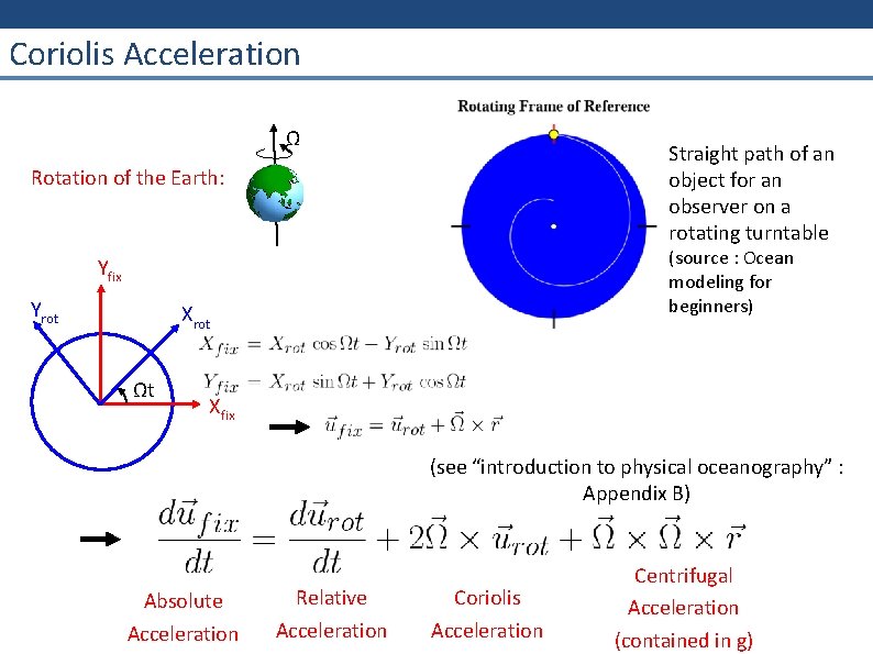
Coriolis Acceleration Ω Straight path of an object for an observer on a rotating turntable Rotation of the Earth: (source : Ocean modeling for beginners) Yfix Yrot Xrot Ωt Xfix (see “introduction to physical oceanography” : Appendix B) Absolute Acceleration Relative Acceleration Coriolis Acceleration Centrifugal Acceleration (contained in g)

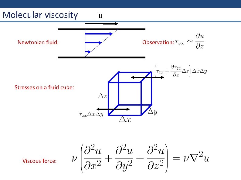
Molecular viscosity Newtonian fluid: Stresses on a fluid cube: Viscous force: U Observation:

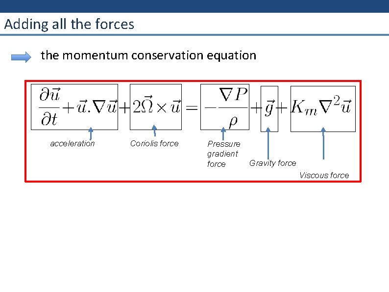
Adding all the forces the momentum conservation equation acceleration Coriolis force Pressure gradient force Gravity force Viscous force

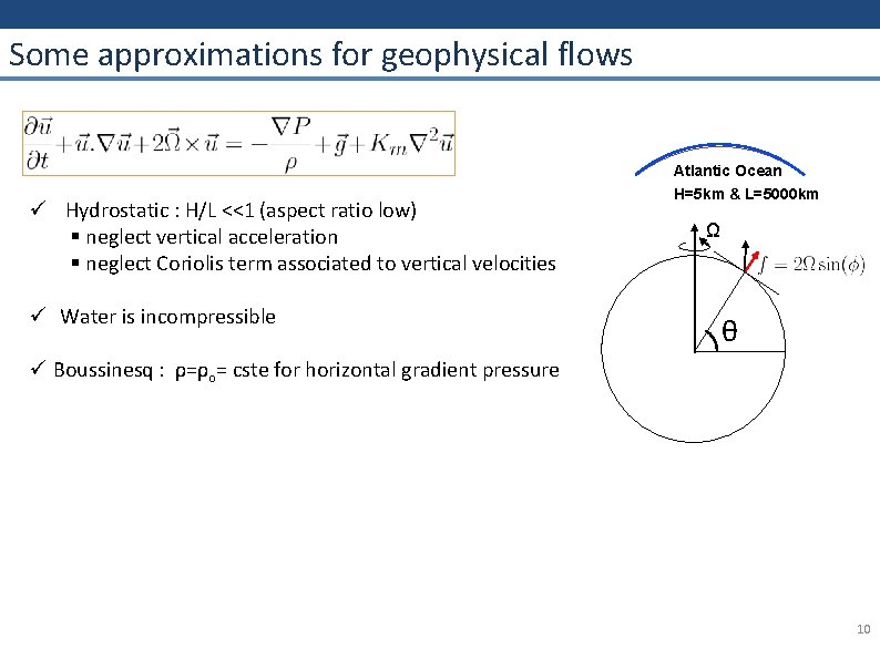
Some approximations for geophysical flows ü Hydrostatic : H/L <<1 (aspect ratio low) § neglect vertical acceleration § neglect Coriolis term associated to vertical velocities ü Water is incompressible Atlantic Ocean H=5 km & L=5000 km Ω θ ü Boussinesq : ρ=ρo= cste for horizontal gradient pressure 10

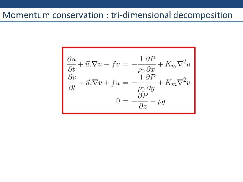
Momentum conservation : tri-dimensional decomposition

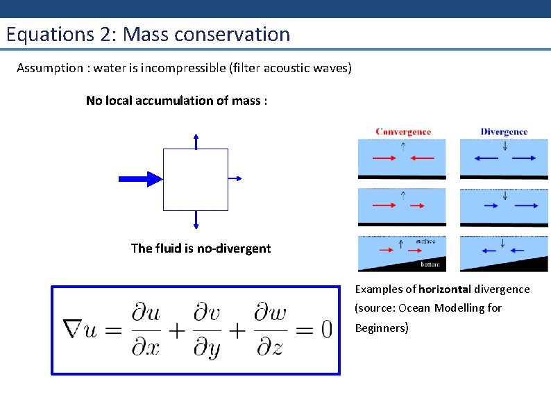
Equations 2: Mass conservation Assumption : water is incompressible (filter acoustic waves) No local accumulation of mass : The fluid is no-divergent Examples of horizontal divergence (source: Ocean Modelling for Beginners)

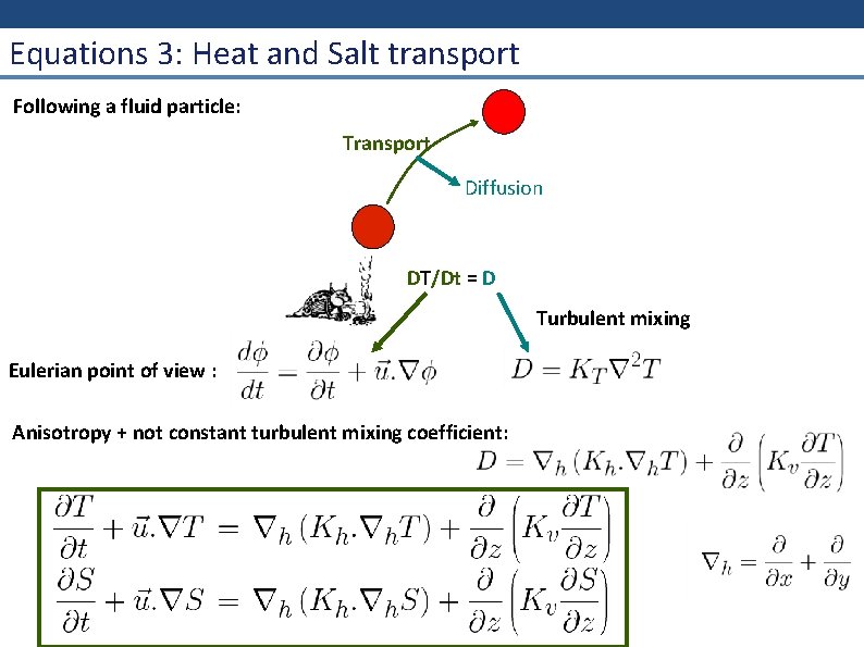
Equations 3: Heat and Salt transport Following a fluid particle: Transport Diffusion DT/Dt = D Turbulent mixing Eulerian point of view : Anisotropy + not constant turbulent mixing coefficient:

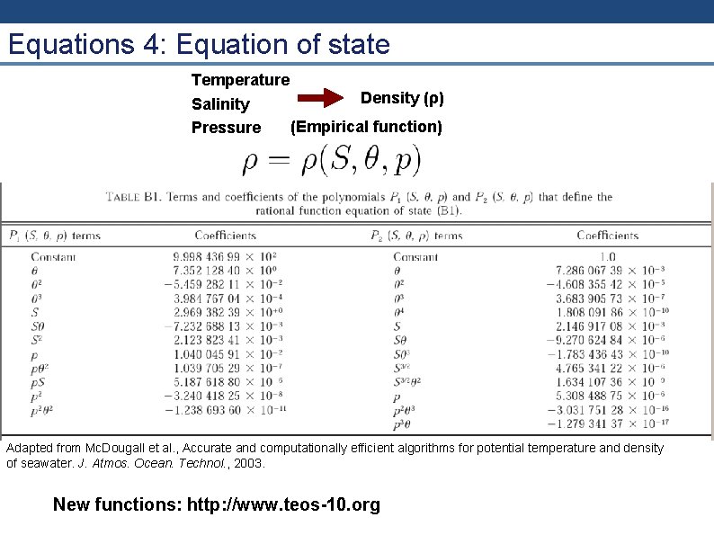
Equations 4: Equation of state Temperature Density (ρ) Salinity (Empirical function) Pressure Adapted from Mc. Dougall et al. , Accurate and computationally efficient algorithms for potential temperature and density of seawater. J. Atmos. Ocean. Technol. , 2003. New functions: http: //www. teos-10. org

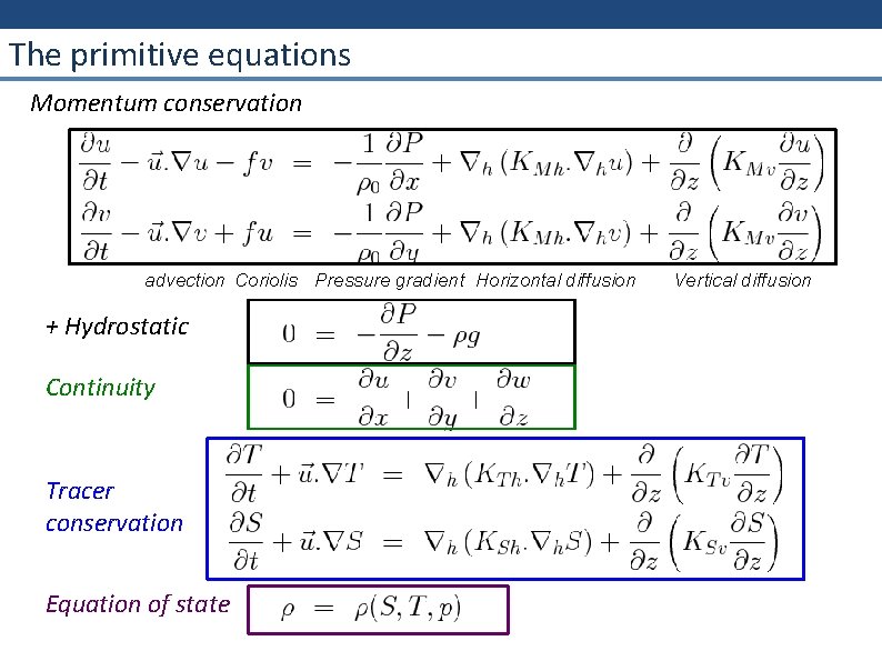
The primitive equations Momentum conservation advection Coriolis Pressure gradient Horizontal diffusion + Hydrostatic Continuity Tracer conservation Equation of state Vertical diffusion

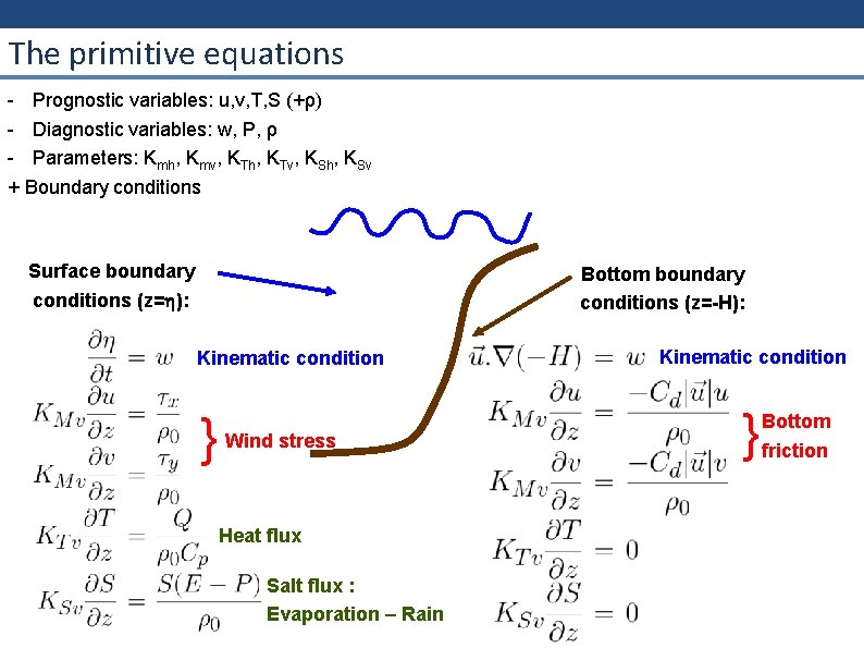
The primitive equations - Prognostic variables: u, v, T, S (+ρ) - Diagnostic variables: w, P, ρ - Parameters: Kmh, Kmv, KTh, KTv, KSh, KSv + Boundary conditions Surface boundary conditions (z= ): Bottom boundary conditions (z=-H): Kinematic condition } Wind stress Heat flux Salt flux : Evaporation – Rain Kinematic condition } Bottom friction