Introduction to Occupancy Models Key to inclass exercise

Introduction to Occupancy Models Key to in-class exercise are in blue Jan 8, 2016 AEC 501 Nathan J. Hostetter njhostet@ncsu. edu 1

Occupancy • Abundance often most interesting variable when analyzing a population • Occupancy – probability that a site is occupied • Probability abundance is >0

Detection/non-detection data • Presence data rise from a two part process • The species occurs in the region of interest AND • The species is discovered by an investigator • What do absence data tell us? • The species does not occur at that particular site OR • The species was not detected by the investigator

Occupancy studies • Introduced by Mac. Kenzie et al. 2002 and Tyre et al. 2003 • Allows for collection of data that is less intensive than those based on abundance estimation • Use a designed survey method like we discussed before – simple random, stratified random, systematic, or double • Multiple site visits are required to estimate detection and probability of occurrence

Why occupancy? • Data to estimate abundance can be difficult to collect, require more time and effort, might be more limited in spatial/temporal scope • Obtaining presence/absence data is • • Usually less intensive Cheaper Can cover a larger area or time frame Might be more practical for certain objectives

Why occupancy? • Some common reasons and objectives • • • Extensive monitoring programs Distribution (e. g. , ranges shifts, invasive species, etc. ) Habitat selection Meta-population dynamics Species interactions Species richness

Occupancy studies • Key design issues: Replication • Temporal replication: • repeat visits to sample units • Spatial replication: • randomly selected ‘sites’ or sample units within area of interest

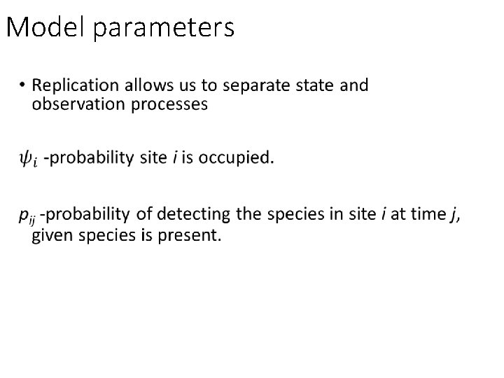
Model parameters

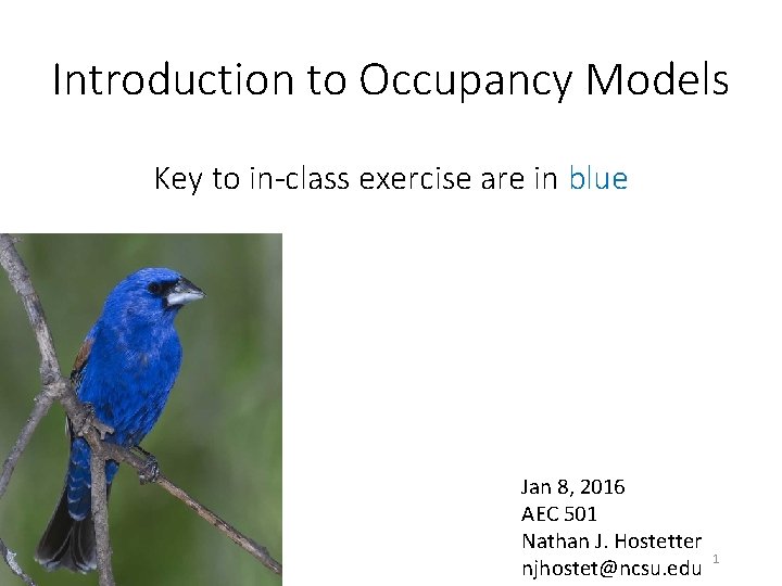
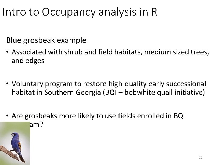
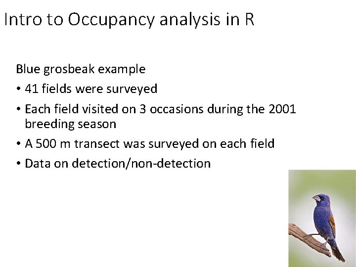
Blue grosbeak example • Associated with shrub and field habitats, medium sized trees, and edges • Voluntary program to restore high-quality early successional habitat in Southern Georgia (BQI – bobwhite quail initiative) • Are grosbeaks more likely to use fields enrolled in BQI program?

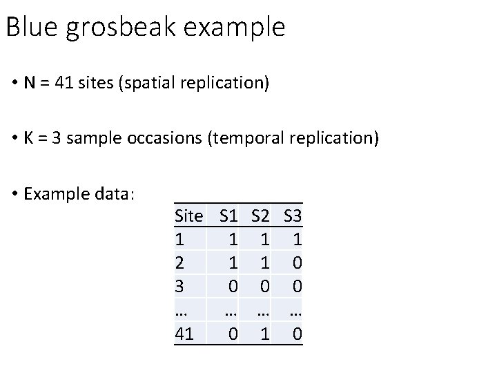
Blue grosbeak example • N = 41 sites (spatial replication) • K = 3 sample occasions (temporal replication) • Example data: Site S 1 S 2 S 3 1 1 2 1 1 0 3 0 0 0 … … 41 0

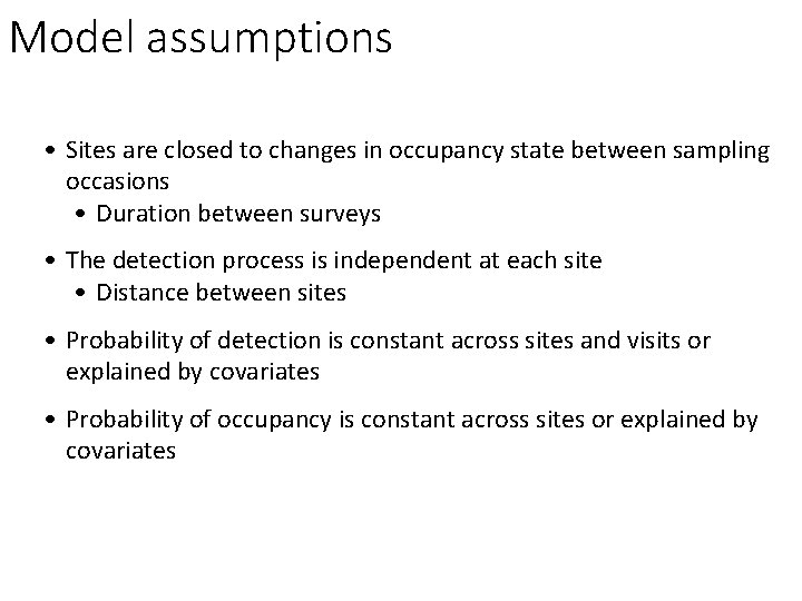
Model assumptions • Sites are closed to changes in occupancy state between sampling occasions • Duration between surveys • The detection process is independent at each site • Distance between sites • Probability of detection is constant across sites and visits or explained by covariates • Probability of occupancy is constant across sites or explained by covariates

Enough talk, Let’s work through the blue grosbeak example

Introduction to R Basics and Occupancy modeling 13

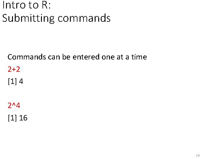
Intro to R: Submitting commands Commands can be entered one at a time 2+2 [1] 4 2^4 [1] 16 14

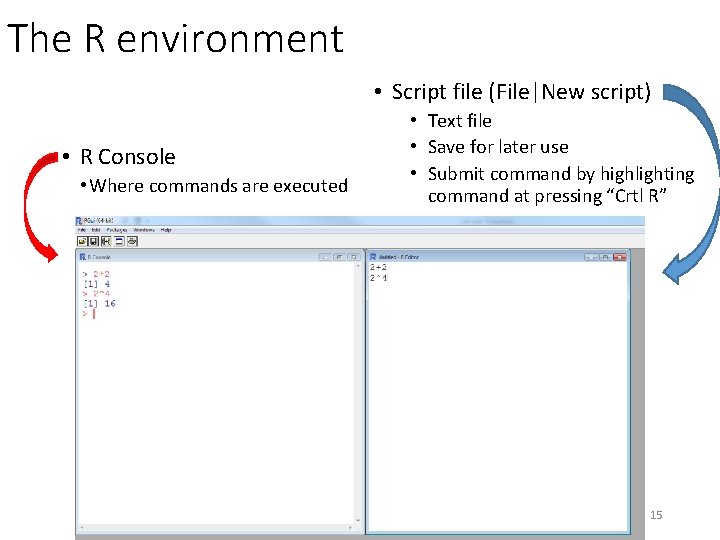
The R environment • Script file (File|New script) • R Console • Where commands are executed • Text file • Save for later use • Submit command by highlighting command at pressing “Crtl R” 15

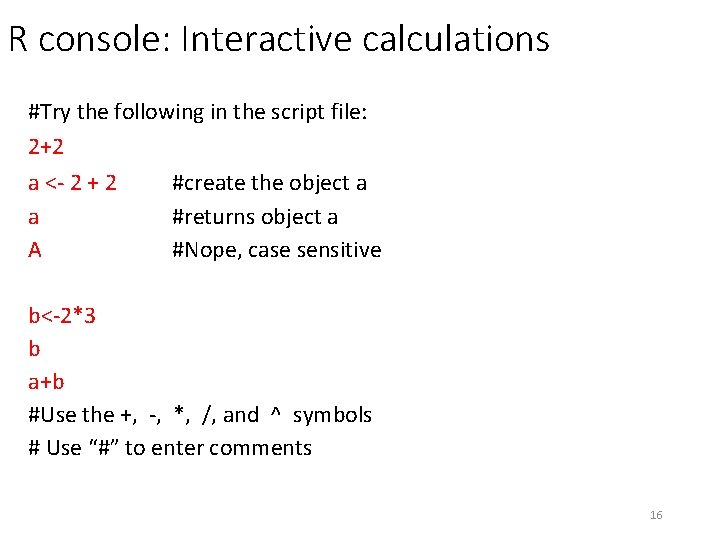
R console: Interactive calculations #Try the following in the script file: 2+2 a <- 2 + 2 #create the object a a #returns object a A #Nope, case sensitive b<-2*3 b a+b #Use the +, -, *, /, and ^ symbols # Use “#” to enter comments 16

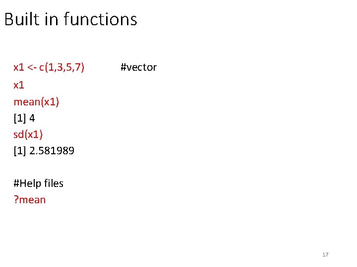
Built in functions x 1 <- c(1, 3, 5, 7) x 1 mean(x 1) [1] 4 sd(x 1) [1] 2. 581989 #vector #Help files ? mean 17

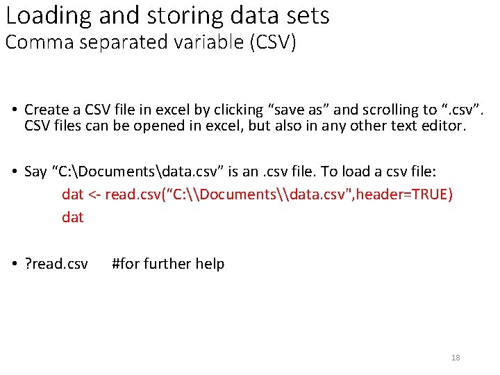
Loading and storing data sets Comma separated variable (CSV) • Create a CSV file in excel by clicking “save as” and scrolling to “. csv”. CSV files can be opened in excel, but also in any other text editor. • Say “C: Documentsdata. csv” is an. csv file. To load a csv file: dat <- read. csv(“C: \Documents\data. csv", header=TRUE) dat • ? read. csv #for further help 18

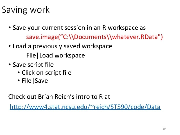
Saving work • Save your current session in an R workspace as save. image(“C: \Documents\whatever. RData") • Load a previously saved workspace File|Load workspace • Save script file • Click on script file • File|Save Check out Brian Reich’s intro to R at http: //www 4. stat. ncsu. edu/~reich/ST 590/code/Data 19

Intro to Occupancy analysis in R Blue grosbeak example • Associated with shrub and field habitats, medium sized trees, and edges • Voluntary program to restore high-quality early successional habitat in Southern Georgia (BQI – bobwhite quail initiative) • Are grosbeaks more likely to use fields enrolled in BQI program? 20

Intro to Occupancy analysis in R Blue grosbeak example • 41 fields were surveyed • Each field visited on 3 occasions during the 2001 breeding season • A 500 m transect was surveyed on each field • Data on detection/non-detection 21

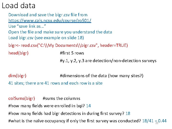
Load data Download and save the blgr. csv file from https: //www. cals. ncsu. edu/course/zo 501/ Use “save link as…” Open the file and make sure you understand the data Load blgr. csv (see example on slide 18) blgr<- read. csv("C: \My Documents\blgr. csv", header=TRUE) head(blgr) #first 5 rows #y. 1, y. 2, y. 3 are detection/non-detection surveys dim(blgr) #dimensions of the data (how many sites? ) 41 sites; there are 41 rows and each row is a site col. Sums(blgr) #sums the columns #how many fields were enrolled in bqi? 14 #how many fields had blgr detections in during first survey? 18 #what is the naïve occupancy if only the first survey was conducted? 18/41 = 0. 44 22

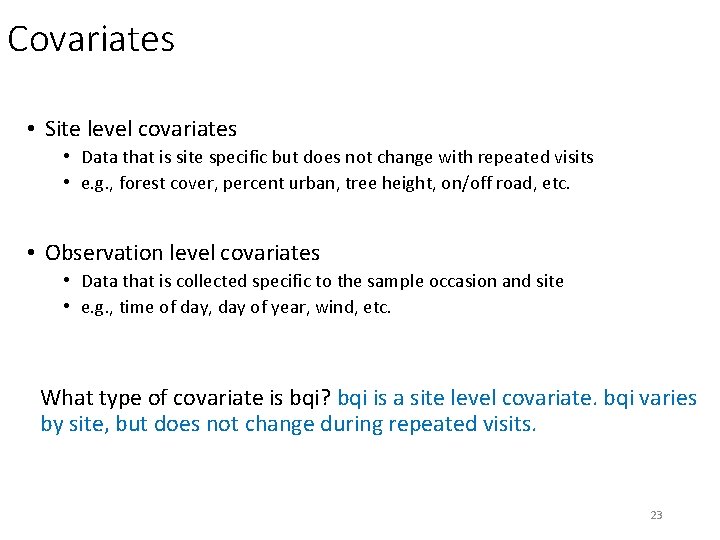
Covariates • Site level covariates • Data that is site specific but does not change with repeated visits • e. g. , forest cover, percent urban, tree height, on/off road, etc. • Observation level covariates • Data that is collected specific to the sample occasion and site • e. g. , time of day, day of year, wind, etc. What type of covariate is bqi? bqi is a site level covariate. bqi varies by site, but does not change during repeated visits. 23

Occupancy analysis – Unmarked • Unmarked • R package • Fits models of animal abundance and occurrence • Complete description of unmarked at https: //cran. rproject. org/web/packages/unmarked. pdf 24

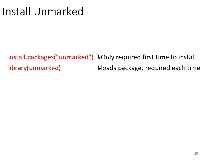
Install Unmarked install. packages("unmarked") #Only required first time to install library(unmarked) #loads package, required each time 25

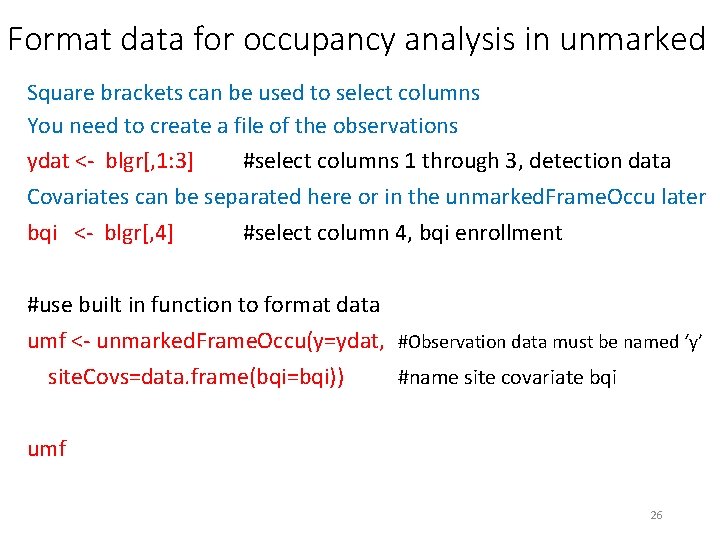
Format data for occupancy analysis in unmarked Square brackets can be used to select columns You need to create a file of the observations ydat <- blgr[, 1: 3] #select columns 1 through 3, detection data Covariates can be separated here or in the unmarked. Frame. Occu later bqi <- blgr[, 4] #select column 4, bqi enrollment #use built in function to format data umf <- unmarked. Frame. Occu(y=ydat, #Observation data must be named ‘y’ site. Covs=data. frame(bqi=bqi)) #name site covariate bqi umf 26

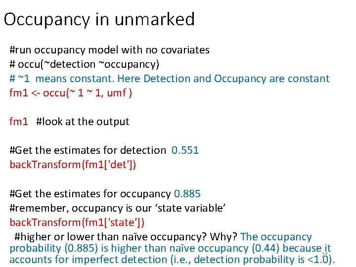
Occupancy in unmarked #run occupancy model with no covariates # occu(~detection ~occupancy) # ~1 means constant. Here Detection and Occupancy are constant fm 1 <- occu(~ 1 ~ 1, umf ) fm 1 #look at the output #Get the estimates for detection 0. 551 back. Transform(fm 1['det']) #Get the estimates for occupancy 0. 885 #remember, occupancy is our ‘state variable’ back. Transform(fm 1['state']) #higher or lower than naïve occupancy? Why? The occupancy probability (0. 885) is higher than naïve occupancy (0. 44) because it 27 accounts for imperfect detection (i. e. , detection probability is <1. 0).

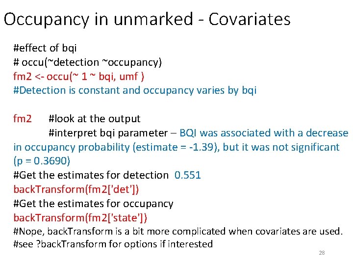
Occupancy in unmarked - Covariates #effect of bqi # occu(~detection ~occupancy) fm 2 <- occu(~ 1 ~ bqi, umf ) #Detection is constant and occupancy varies by bqi fm 2 #look at the output #interpret bqi parameter – BQI was associated with a decrease in occupancy probability (estimate = -1. 39), but it was not significant (p = 0. 3690) #Get the estimates for detection 0. 551 back. Transform(fm 2['det']) #Get the estimates for occupancy back. Transform(fm 2['state']) #Nope, back. Transform is a bit more complicated when covariates are used. #see ? back. Transform for options if interested 28

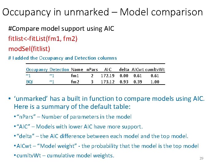
Occupancy in unmarked – Model comparison #Compare model support using AIC fitlist<-fit. List(fm 1, fm 2) mod. Sel(fitlist) # I added the Occupancy and Detection columns Occupancy Detection Name n. Pars AIC delta AICwt cumltv. Wt ~1 ~1 fm 1 2 172. 19 0. 00 0. 61 BQI ~1 fm 2 3 173. 12 0. 93 0. 39 1. 00 • ‘unmarked’ has a built in function to compare models using AIC. Here is a summary of the default table: • “n. Pars” – Number of parameters in the model • “AIC” – Models with lower AIC have more support. • “delta” – the AIC difference between each model and the top model. • AICwt – “Model weight” - the probability that the model is the top model • cumltv. Wt – cumulative model weights. 29

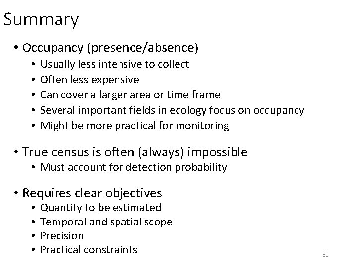
Summary • Occupancy (presence/absence) • • • Usually less intensive to collect Often less expensive Can cover a larger area or time frame Several important fields in ecology focus on occupancy Might be more practical for monitoring • True census is often (always) impossible • Must account for detection probability • Requires clear objectives • • Quantity to be estimated Temporal and spatial scope Precision Practical constraints 30

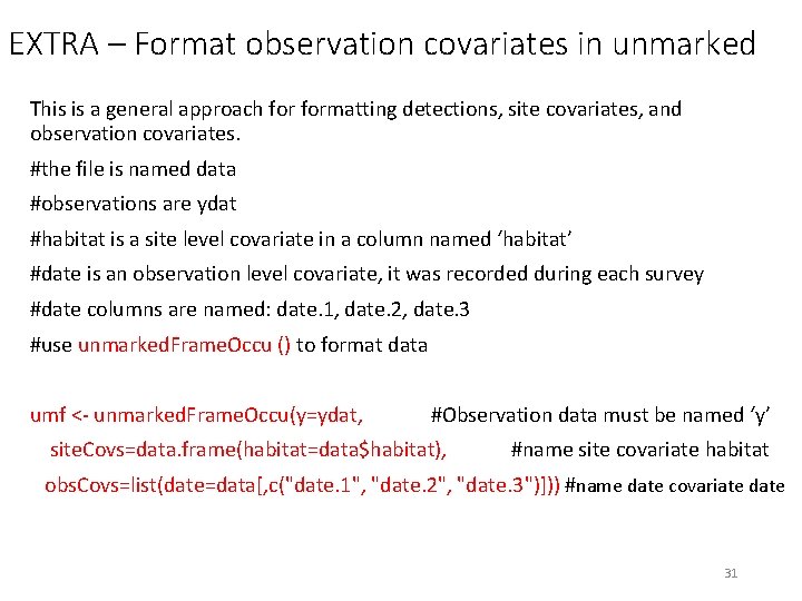
EXTRA – Format observation covariates in unmarked This is a general approach formatting detections, site covariates, and observation covariates. #the file is named data #observations are ydat #habitat is a site level covariate in a column named ‘habitat’ #date is an observation level covariate, it was recorded during each survey #date columns are named: date. 1, date. 2, date. 3 #use unmarked. Frame. Occu () to format data umf <- unmarked. Frame. Occu(y=ydat, #Observation data must be named ‘y’ site. Covs=data. frame(habitat=data$habitat), #name site covariate habitat obs. Covs=list(date=data[, c("date. 1", "date. 2", "date. 3")])) #name date covariate date 31