Introduction to NLP Mathematical Foundations Probability Many slides
Introduction to NLP Mathematical Foundations: Probability Many slides reused from Barbara Rosario (UC Berkeley)

Motivations • Statistical NLP aims to do statistical inference for the field of NL • Statistical inference consists of taking some data (generated in accordance with some unknown probability distribution) and then making some inference about this distribution. 2 3/4/2021
Motivations (Cont) • An example of statistical inference is the task of language modeling (ex how to predict the next word given the previous words) • In order to do this, we need a model of the language. • Probability theory helps us finding such model 3 3/4/2021
Probability Theory • How likely it is that something will happen • Sample space Ω is listing of all possible outcomes of an experiment • P(Ω) = 1 • Any experimental outcome ω must be within Ω • P(ω) = [0, 1] 4 3/4/2021
Events • Event A is a subset of Ω • An event is a set of outcomes • Probability function (or distribution) • maps from each of the events in Ω to its probability 5 3/4/2021
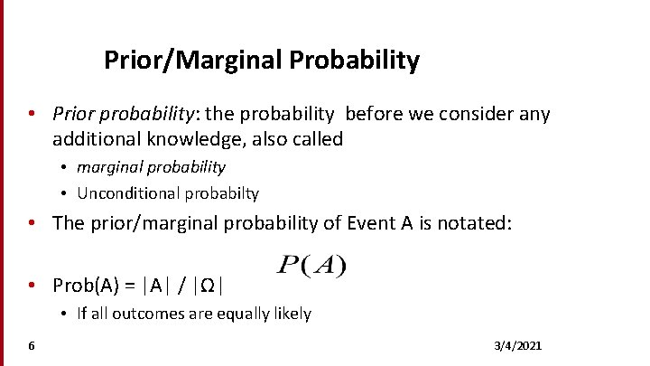
Prior/Marginal Probability • Prior probability: the probability before we consider any additional knowledge, also called • marginal probability • Unconditional probabilty • The prior/marginal probability of Event A is notated: • Prob(A) = |A| / |Ω| • If all outcomes are equally likely 6 3/4/2021
Probability Example • Experimental Protocol: Flip a fair coin 3 times • Ω: set of all HT combinations of length 3 • {HHH, HHT, HTH, HTT, THH, THT, TTH, TTT} • Each of the 8 basic outcomes is equally likely with probability of 1/8 • Event A: a subset of Ω, e. g. , getting 2 H and 1 T in any order • {HHT, HTH, THH} • Prob(A) = |A| / |Ω| = 3/8 = 0. 375 or 37. 5% 7

Disjoint Events • Probabilities are countably additive for disjoint events • P (A or B) = P(A) + P(B) 8
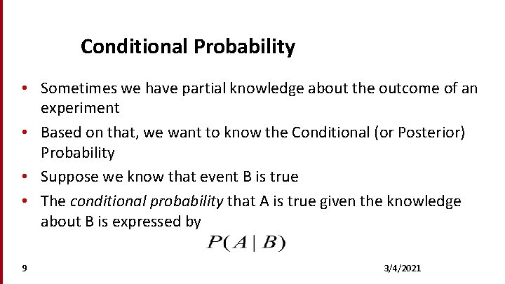
Conditional Probability • Sometimes we have partial knowledge about the outcome of an experiment • Based on that, we want to know the Conditional (or Posterior) Probability • Suppose we know that event B is true • The conditional probability that A is true given the knowledge about B is expressed by 9 3/4/2021
Conditional Probability (independent) • If A and B are independent, then • P (A | B) = P (A) • i. e. , knowing that B has happened does not change P(A) • E. g. , P (H | T) = 50% == P(H) • When flipping a fair coin, previous events don’t affect future probabilities 10

Conditional Probability (dependent Example) • Event B: First coin flipped is a H • What is P (A|B)? • Ω’: set of all HT combinations of length 3 starting with H • {HHH, HHT, HTH, HTT} • A’: {HHT, HTH} • P(A|B) = |A’|/|Ω’| = 2/4 = 50% • Contrast with P(A) = 37. 5%; knowing that B has happened has boosted the likelihood of A happening 11
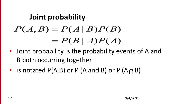
Joint probability • Joint probability is the probability events of A and B both occurring together • is notated P(A, B) or P (A and B) or P (A B) U 12 3/4/2021
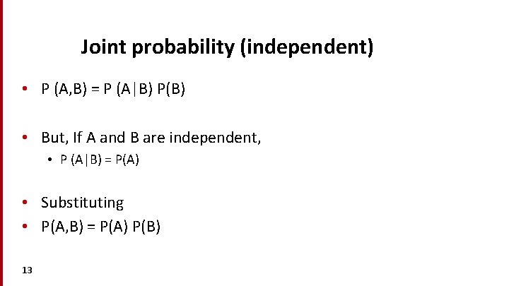
Joint probability (independent) • P (A, B) = P (A|B) P(B) • But, If A and B are independent, • P (A|B) = P(A) • Substituting • P(A, B) = P(A) P(B) 13
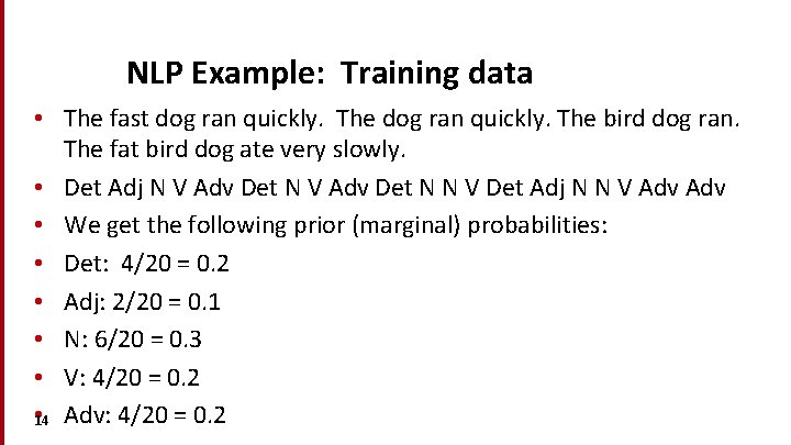
NLP Example: Training data • The fast dog ran quickly. The bird dog ran. The fat bird dog ate very slowly. • Det Adj N V Adv Det N N V Det Adj N N V Adv • We get the following prior (marginal) probabilities: • Det: 4/20 = 0. 2 • Adj: 2/20 = 0. 1 • N: 6/20 = 0. 3 • V: 4/20 = 0. 2 • Adv: 4/20 = 0. 2 14
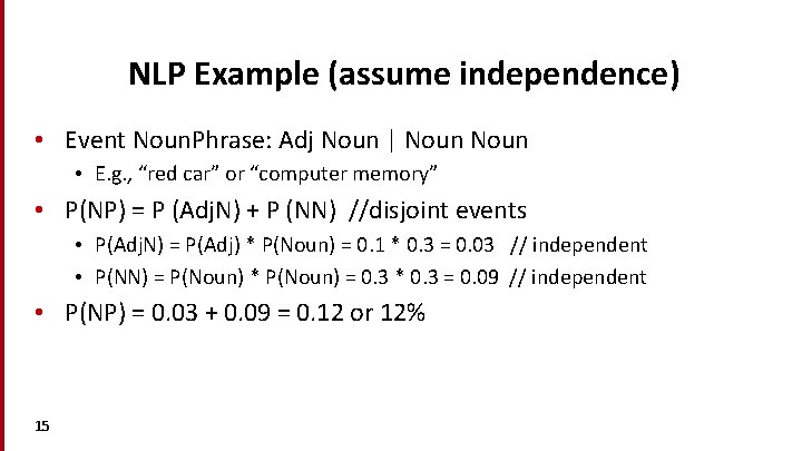
NLP Example (assume independence) • Event Noun. Phrase: Adj Noun | Noun • E. g. , “red car” or “computer memory” • P(NP) = P (Adj. N) + P (NN) //disjoint events • P(Adj. N) = P(Adj) * P(Noun) = 0. 1 * 0. 3 = 0. 03 // independent • P(NN) = P(Noun) * P(Noun) = 0. 3 * 0. 3 = 0. 09 // independent • P(NP) = 0. 03 + 0. 09 = 0. 12 or 12% 15
Joint probability (dependent) • If A and B are not independent, P (A, B) is represented using a 2 -dimensional table with a value in every cell giving the probability of that specific state occurring based on training data • Values are set using training data 16 3/4/2021
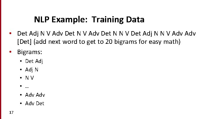
NLP Example: Training Data • Det Adj N V Adv Det N N V Det Adj N N V Adv [Det] (add next word to get to 20 bigrams for easy math) • Bigrams: • • • 17 Det Adj N NV … Adv Adv Det
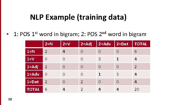
NLP Example (training data) • 1: POS 1 st word in bigram; 2: POS 2 nd word in bigram 18 2=N 2=V 2=Adj 2=Adv 2=Det TOTAL 1=N 2 4 0 0 0 6 1=V 0 0 0 3 1 4 1=Adj 2 0 0 2 1=Adv 0 0 0 1 3 4 1=Det 2 0 0 4 TOTAL 6 4 2 4 4 20
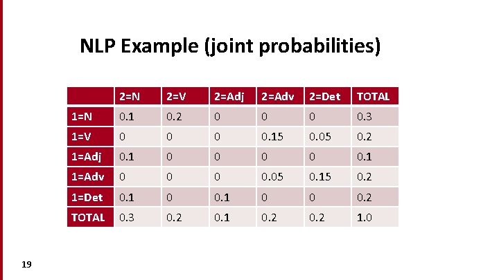
NLP Example (joint probabilities) 19 2=N 2=V 2=Adj 2=Adv 2=Det TOTAL 1=N 0. 1 0. 2 0 0. 3 1=V 0 0. 15 0. 05 0. 2 1=Adj 0. 1 0 0 0. 1 1=Adv 0 0. 05 0. 15 0. 2 1=Det 0. 1 0 0 0. 2 TOTAL 0. 3 0. 2 0. 1 0. 2 1. 0
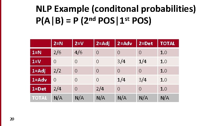
NLP Example (conditonal probabilities) P(A|B) = P (2 nd POS|1 st POS) 20 2=N 2=V 2=Adj 2=Adv 2=Det TOTAL 1=N 2/6 4/6 0 0 0 1=V 0 0 0 3/4 1. 0 1=Adj 2/2 0 0 1=Adv 0 0 0 1/4 3/4 1. 0 1=Det 2/4 0 0 1. 0 TOTAL N/A N/A N/A
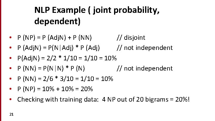
NLP Example ( joint probability, dependent) • • 21 P (NP) = P (Adj. N) + P (NN) // disjoint P (Adj. N) = P(N|Adj) * P (Adj) // not independent P(Adj. N) = 2/2 * 1/10 = 10% P (NN) = P(N|N) * P (N) // not independent P (NN) = 2/6 * 3/10 = 10% P (NP) = 10% + 10% = 20% Checking with training data: 4 NP out of 20 bigrams = 20%!
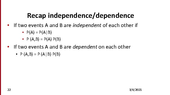
Recap independence/dependence • If two events A and B are independent of each other if • P(A) = P(A|B) • P (A, B) = P(A) P(B) • If two events A and B are dependent on each other • P (A, B) = P (A|B) P(B) 22 3/4/2021
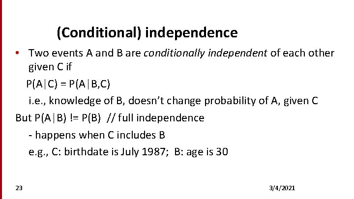
(Conditional) independence • Two events A and B are conditionally independent of each other given C if P(A|C) = P(A|B, C) i. e. , knowledge of B, doesn’t change probability of A, given C But P(A|B) != P(B) // full independence - happens when C includes B e. g. , C: birthdate is July 1987; B: age is 30 23 3/4/2021
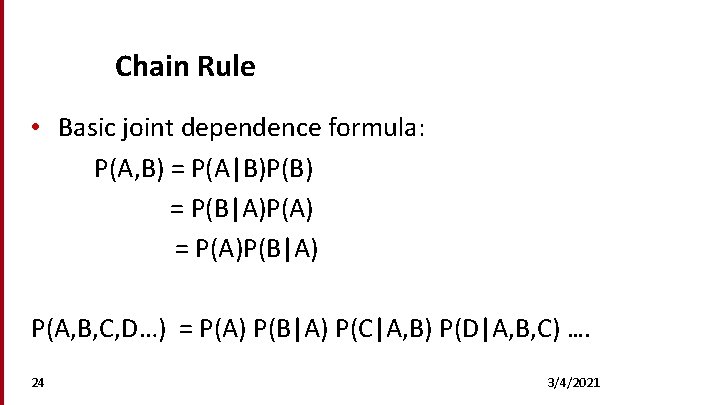
Chain Rule • Basic joint dependence formula: P(A, B) = P(A|B)P(B) = P(B|A)P(A) = P(A)P(B|A) P(A, B, C, D…) = P(A) P(B|A) P(C|A, B) P(D|A, B, C) …. 24 3/4/2021
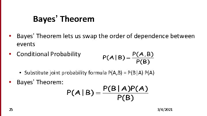
Bayes’ Theorem • Bayes’ Theorem lets us swap the order of dependence between events • Conditional Probability • Substitute joint probability formula P(A, B) = P(B|A) P(A) • Bayes’ Theorem: 25 3/4/2021
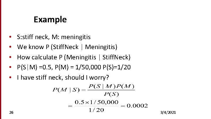
Example • • • 26 S: stiff neck, M: meningitis We know P (Stiff. Neck | Meningitis) How calculate P (Meningitis | Stiff. Neck) P(S|M) =0. 5, P(M) = 1/50, 000 P(S)=1/20 I have stiff neck, should I worry? 3/4/2021
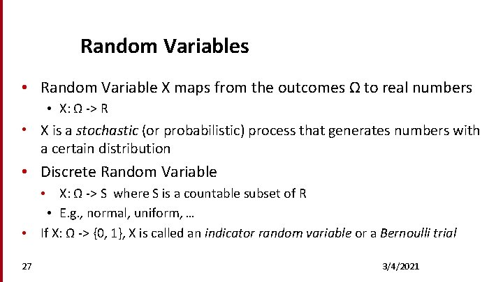
Random Variables • Random Variable X maps from the outcomes Ω to real numbers • X: Ω -> R • X is a stochastic (or probabilistic) process that generates numbers with a certain distribution • Discrete Random Variable • X: Ω -> S where S is a countable subset of R • E. g. , normal, uniform, … • If X: Ω -> {0, 1}, X is called an indicator random variable or a Bernoulli trial 27 3/4/2021
Probability Mass Function (pmf) • The probability mass function (pmf) for random variable X gives the probability that X has various values • i. e. , study values of X (which may be fewer) rather than outcomes of events • The sum of the pmf must be 1. 0 28
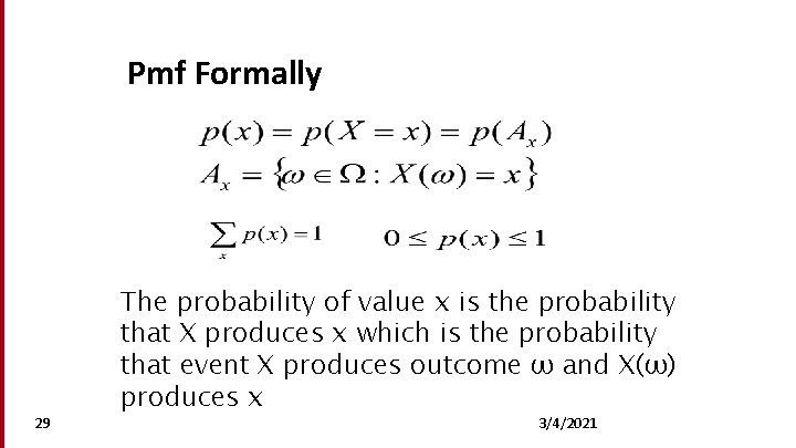
Pmf Formally 29 The probability of value x is the probability that X produces x which is the probability that event X produces outcome ω and X(ω) produces x 3/4/2021
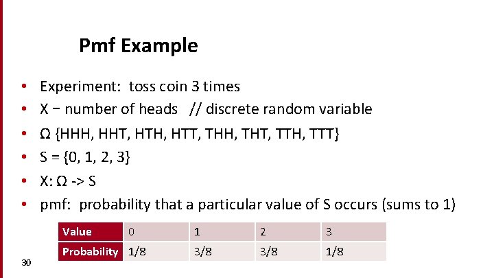
Pmf Example • • • Experiment: toss coin 3 times X – number of heads // discrete random variable Ω {HHH, HHT, HTH, HTT, THH, THT, TTH, TTT} S = {0, 1, 2, 3} X: Ω -> S pmf: probability that a particular value of S occurs (sums to 1) Value 30 0 Probability 1/8 1 2 3 3/8 1/8
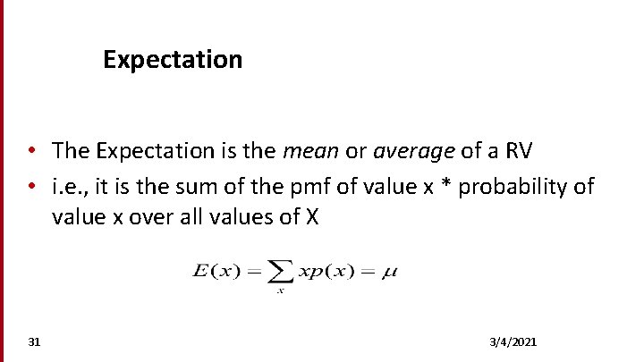
Expectation • The Expectation is the mean or average of a RV • i. e. , it is the sum of the pmf of value x * probability of value x over all values of X 31 3/4/2021
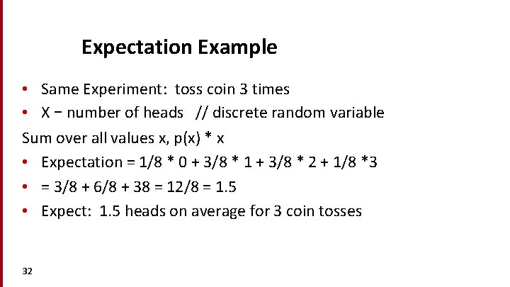
Expectation Example • Same Experiment: toss coin 3 times • X – number of heads // discrete random variable Sum over all values x, p(x) * x • Expectation = 1/8 * 0 + 3/8 * 1 + 3/8 * 2 + 1/8 *3 • = 3/8 + 6/8 + 38 = 12/8 = 1. 5 • Expect: 1. 5 heads on average for 3 coin tosses 32
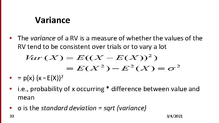
Variance • The variance of a RV is a measure of whether the values of the RV tend to be consistent over trials or to vary a lot • = p(x) (x – E(X))2 • i. e. , probability of x occurring * difference between value and mean • σ is the standard deviation = sqrt (variance) 33 3/4/2021
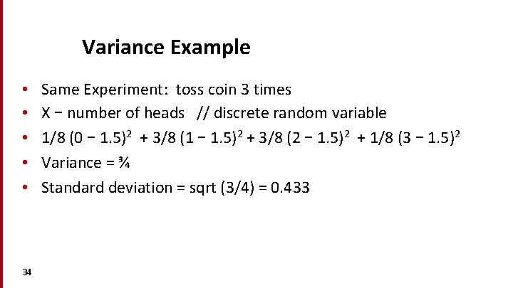
Variance Example • • • 34 Same Experiment: toss coin 3 times X – number of heads // discrete random variable 1/8 (0 – 1. 5)2 + 3/8 (1 – 1. 5)2 + 3/8 (2 – 1. 5)2 + 1/8 (3 – 1. 5)2 Variance = ¾ Standard deviation = sqrt (3/4) = 0. 433
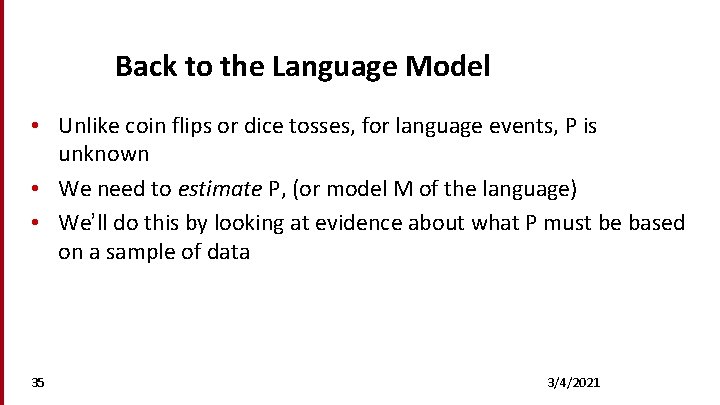
Back to the Language Model • Unlike coin flips or dice tosses, for language events, P is unknown • We need to estimate P, (or model M of the language) • We’ll do this by looking at evidence about what P must be based on a sample of data 35 3/4/2021
Estimation of P • Frequentist statistics • Bayesian statistics 36 3/4/2021
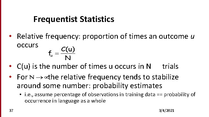
Frequentist Statistics • Relative frequency: proportion of times an outcome u occurs • C(u) is the number of times u occurs in N trials • For the relative frequency tends to stabilize around some number: probability estimates • i. e. , assume percentage of observations in training data == probability of occurrence in language as a whole 37 3/4/2021
Frequentist Statistics (cont) • Two different approach: • Parametric • Non-parametric (distribution free) 38 3/4/2021
Parametric Methods • Assume that some phenomenon in language is acceptably modeled by one of the well-known family of distributions (such binomial, normal) • We have an explicit probabilistic model of the process by which the data was generated, and determining a particular probability distribution within the family requires only the specification of a few parameters (less training data) 39 3/4/2021
Non-Parametric Methods • No assumption about the underlying distribution of the data • E. g. , simply estimate P empirically by counting a large number of random events is a distribution-free method • Less prior information, more training data needed 40 3/4/2021
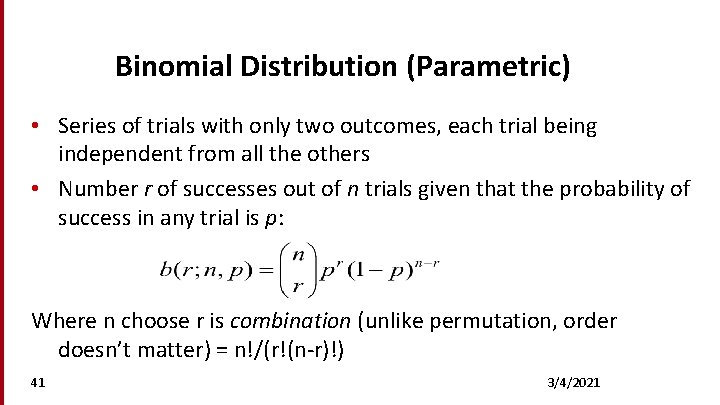
Binomial Distribution (Parametric) • Series of trials with only two outcomes, each trial being independent from all the others • Number r of successes out of n trials given that the probability of success in any trial is p: Where n choose r is combination (unlike permutation, order doesn’t matter) = n!/(r!(n-r)!) 41 3/4/2021
Binomial Distribution Example • “Modeling Public Mood and Emotion: Twitter Sentiment and Socio-Economic Phenomena” • https: //www. aaai. org/ocs/index. php/ICWSM 11/paper/view. File/2 826/3237 • “The probability that the terms extracted from the tweets submitted on any given day match the given number of POMS adjectives Np thus varies considerably along the binomial probability mass function… where P(K=n) represents the probability of achieving n number of POMS term matches. ” 42
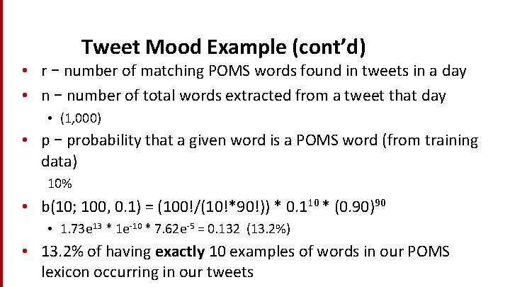
Tweet Mood Example (cont’d) • r – number of matching POMS words found in tweets in a day • n – number of total words extracted from a tweet that day • (1, 000) • p – probability that a given word is a POMS word (from training data) 10% • b(10; 100, 0. 1) = (100!/(10!*90!)) * 0. 110 * (0. 90)90 • 1. 73 e 13 * 1 e-10 * 7. 62 e-5 = 0. 132 (13. 2%) • 13. 2% of having exactly 10 examples of words in our POMS lexicon occurring in our tweets
Tweet Mood Example (cont’d) • What about having at least 10 words from our POMS lexicon being found? • Need to do 1 – (SUM of 0. . 9 words exactly) • Get: 1 – 0. 451 = 54. 8% of the time we can expect at least 10 POMS word occurrences • How get a better hit rate? • Make our lexicon bigger! If probability of being in the lexicon is 20%, then we get 99. 8% of the days above our threshold • Collect more data! If we collect 2000 words per day, we get 99. 6% of the days above our threshold
About binomial distributions • Used in counting n-grams, hypothesis testing • If more than 2 outcomes, called multinomial distribution • Other useful discrete distributions • Poisson (events with known average rate, but independent occurrences) • E. g. , distribution of words across documents (somewhat accurate for non-content words, not accurate for content-bearing words) • Bernoulli (binomial with only 1 trial) 45
Normal (Gaussian) Distribution (Parametric) • Continuous distribution (i. e. , Not discrete) • Two parameters: mean μ and standard deviation σ • May be used to approximate discrete binomial distributions • Many clustering algorithms are based on Gaussian distributions 46 3/4/2021
Other continuous distributions • t distribution used in hypothesis testing • Student’s t test 47
Bayesian Statistics • Bayesian statistics measures degrees of belief • Degrees are calculated by starting with prior beliefs and updating them in face of the evidence, using Bayes theorem 48 3/4/2021
Bayesian Updating • We start with a priori probability distribution P(M) • When a new datum comes in, we update our beliefs by calculating the posterior probability P(M|D). • This then becomes the new prior and the process repeats on each new datum 49 3/4/2021
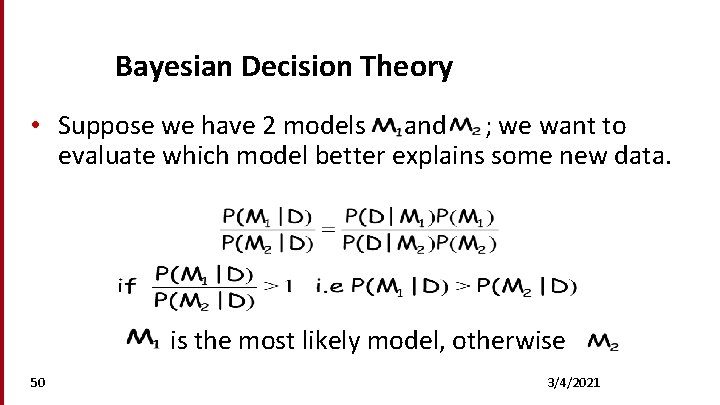
Bayesian Decision Theory • Suppose we have 2 models and ; we want to evaluate which model better explains some new data. is the most likely model, otherwise 50 3/4/2021
Introduction to NLP Mathematical Foundations: Probability
- Slides: 51