Introduction to Neural Networks Dr David Wong with

Introduction to Neural Networks Dr David Wong (with thanks to Dr Gari Clifford, G. I. T)

Overview • What are Artificial Neural Networks (ANNs)? • How do you construct them? • Choosing architecture • Pruning • How do you train them? • Balancing data • Overfitting • Optimization • N-fold Cross Validation

Other Resources • Pattern Recognition and Machine Learning, Chp 5.

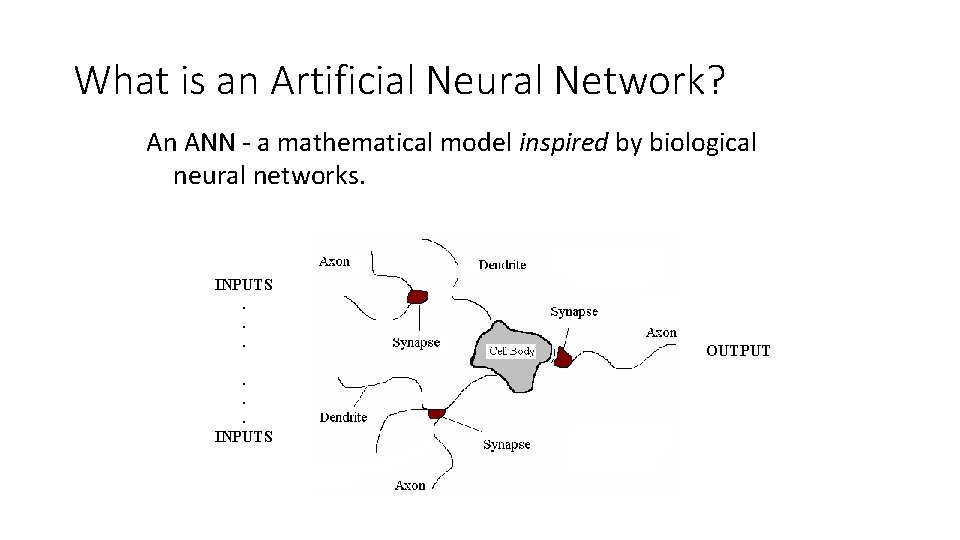
What is an Artificial Neural Network? An ANN - a mathematical model inspired by biological neural networks. INPUTS. . . INPUTS OUTPUT

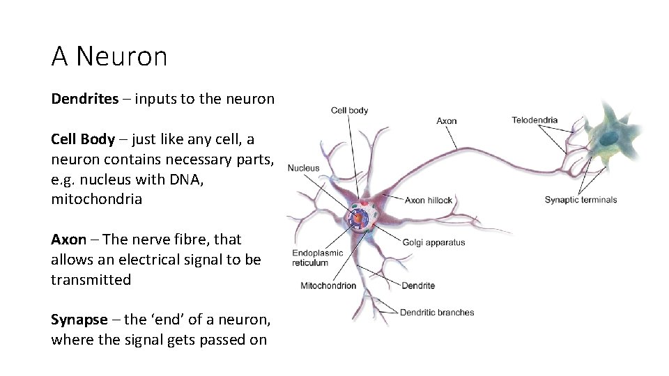
A Neuron Dendrites – inputs to the neuron Cell Body – just like any cell, a neuron contains necessary parts, e. g. nucleus with DNA, mitochondria Axon – The nerve fibre, that allows an electrical signal to be transmitted Synapse – the ‘end’ of a neuron, where the signal gets passed on

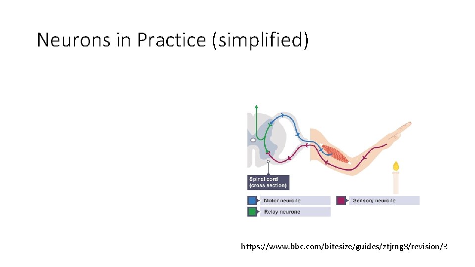
Neurons in Practice (simplified) https: //www. bbc. com/bitesize/guides/ztjrng 8/revision/3

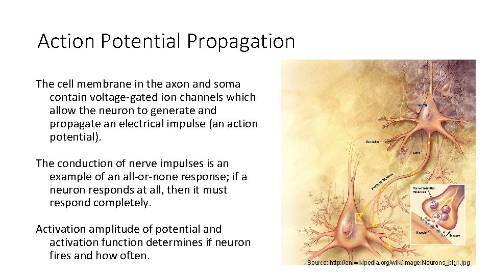
Action Potential Propagation The cell membrane in the axon and soma contain voltage-gated ion channels which allow the neuron to generate and propagate an electrical impulse (an action potential). The conduction of nerve impulses is an example of an all-or-none response; if a neuron responds at all, then it must respond completely. Activation amplitude of potential and activation function determines if neuron fires and how often. Source: http: //en. wikipedia. org/wiki/Image: Neurons_big 1. jpg

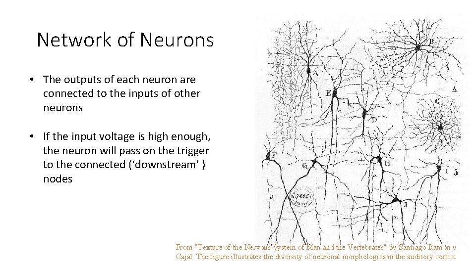
Network of Neurons • The outputs of each neuron are connected to the inputs of other neurons • If the input voltage is high enough, the neuron will pass on the trigger to the connected (‘downstream’ ) nodes From "Texture of the Nervous System of Man and the Vertebrates" by Santiago Ramón y Cajal. The figure illustrates the diversity of neuronal morphologies in the auditory cortex.

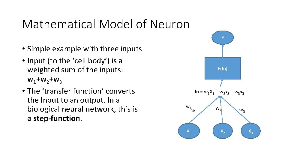
Mathematical Model of Neuron Y • Simple example with three inputs • Input (to the ‘cell body’) is a weighted sum of the inputs: w 1+w 2+w 3 • The ‘transfer function‘ converts the Input to an output. In a biological neural network, this is a step-function. F(In) In = w 1 X 1 + w 2 x 2 + w 3 x 3 w 1 X 1 w 2 X 2 w 3 X 3

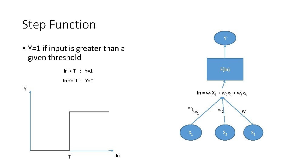
Step Function Y • Y=1 if input is greater than a given threshold F(In) In > T : Y=1 In <= T : Y=0 Y In = w 1 X 1 + w 2 x 2 + w 3 x 3 w 1 X 1 T In w 2 X 2 w 3 X 3

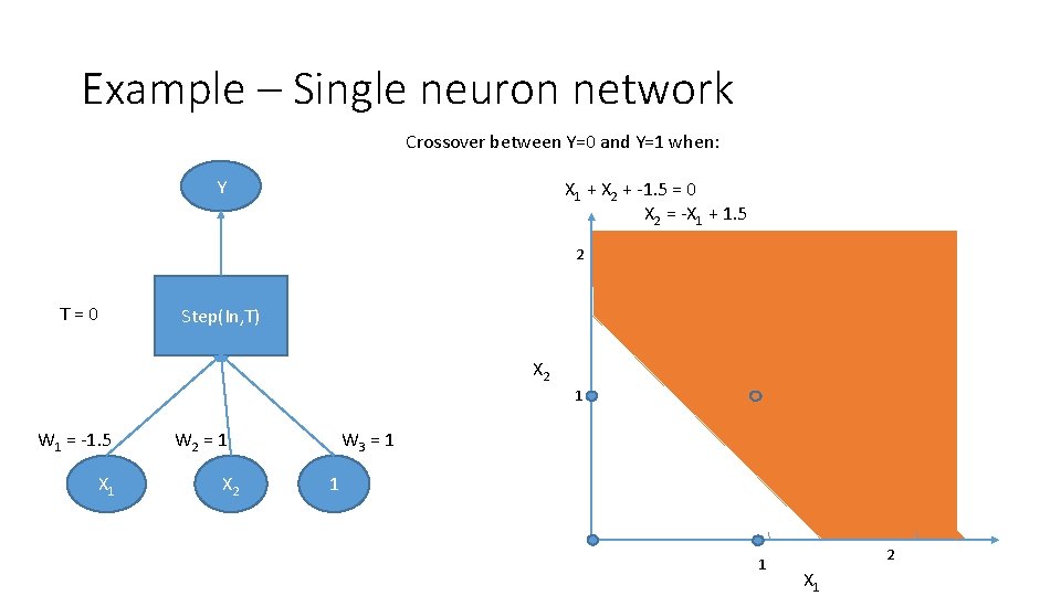
Example – Single neuron network Crossover between Y=0 and Y=1 when: Y X 1 + X 2 + -1. 5 = 0 X 2 = -X 1 + 1. 5 2 T=0 Step(In, T) X 2 1 W 1 = -1. 5 X 1 W 2 = 1 X 2 W 3 = 1 1 1 2 X 1

Example – Single neuron network • In fact, this three input, one output network can be used to model any linear classifier for two independent features variables • (why do you think this is true? ) • To model more complicated classification boundaries, we combine these elementary neurons into more complicated networks

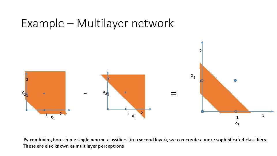
Example – Multilayer network 2 X 2 2 2 - X 2 1 1 X 1 2 1 = X 2 1 1 X 1 2 X 1 By combining two simple single neuron classifiers (in a second layer), we can create a more sophisticated classifiers. These are also known as multilayer perceptrons

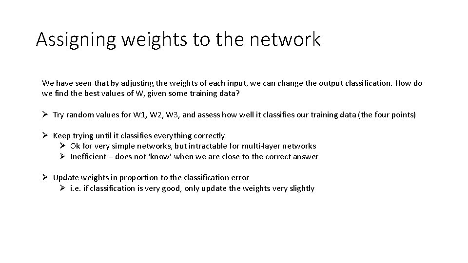
Assigning weights to the network We have seen that by adjusting the weights of each input, we can change the output classification. How do we find the best values of W, given some training data? Ø Try random values for W 1, W 2, W 3, and assess how well it classifies our training data (the four points) Ø Keep trying until it classifies everything correctly Ø Ok for very simple networks, but intractable for multi-layer networks Ø Inefficient – does not ‘know’ when we are close to the correct answer Ø Update weights in proportion to the classification error Ø i. e. if classification is very good, only update the weights very slightly

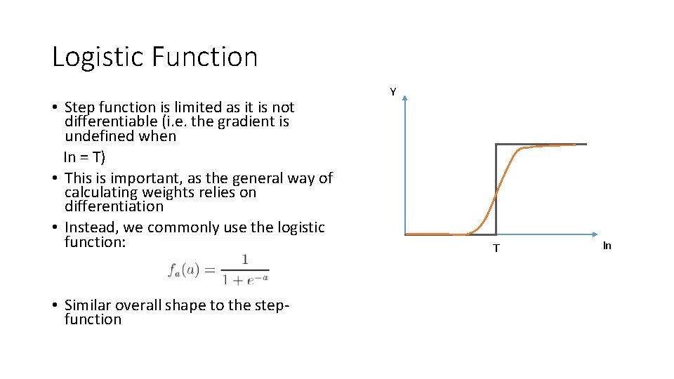
Logistic Function • Step function is limited as it is not differentiable (i. e. the gradient is undefined when In = T) • This is important, as the general way of calculating weights relies on differentiation • Instead, we commonly use the logistic function: • Similar overall shape to the stepfunction Y T In

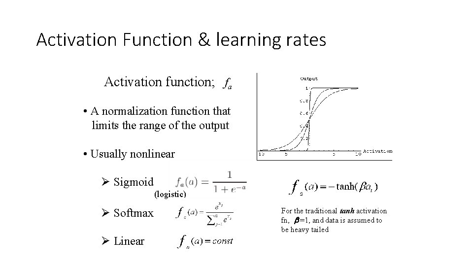
Activation Function & learning rates Activation function; fa • A normalization function that limits the range of the output • Usually nonlinear Ø Sigmoid (logistic) Ø Softmax Ø Linear For the traditional tanh activation fn, =1, and data is assumed to be heavy tailed

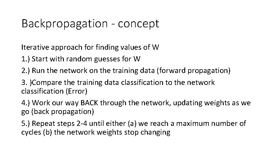
Backpropagation - concept Iterative approach for finding values of W 1. ) Start with random guesses for W 2. ) Run the network on the training data (forward propagation) 3. )Compare the training data classification to the network classification (Error) 4. ) Work our way BACK through the network, updating weights as we go (back propagation) 5. ) Repeat steps 2 -4 until either (a) we reach a maximum number of cycles (b) the network weights stop changing

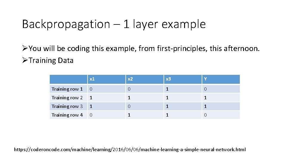
Backpropagation – 1 layer example ØYou will be coding this example, from first-principles, this afternoon. ØTraining Data x 1 x 2 x 3 Y Training row 1 0 0 1 0 Training row 2 1 1 Training row 3 1 0 1 1 Training row 4 0 1 1 0 https: //coderoncode. com/machine/learning/2016/06/06/machine-learning-a-simple-neural-network. html

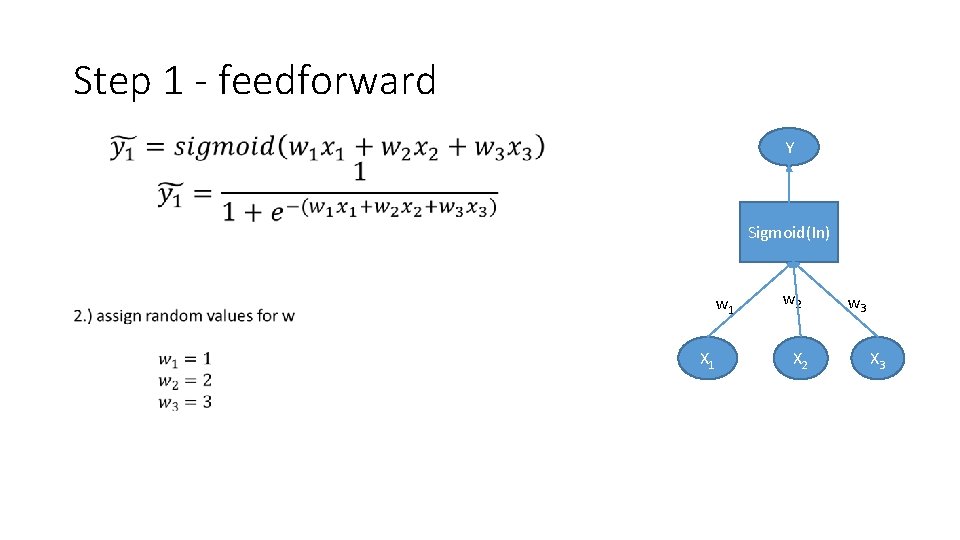
Step 1 - feedforward • Y Sigmoid(In) w 1 X 1 w 2 X 2 w 3 X 3

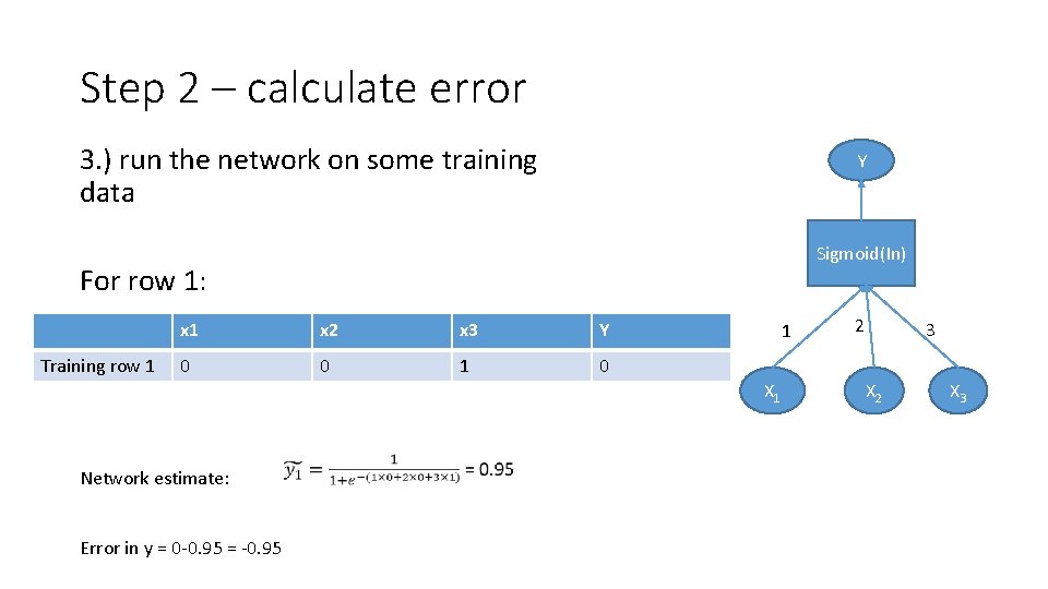
Step 2 – calculate error 3. ) run the network on some training data Y Sigmoid(In) For row 1: Training row 1 x 2 x 3 Y 0 0 1 X 1 Network estimate: Error in y = 0 -0. 95 = -0. 95 2 3 X 2 X 3

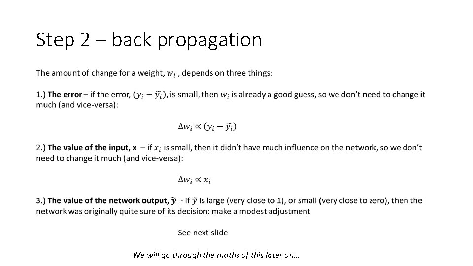
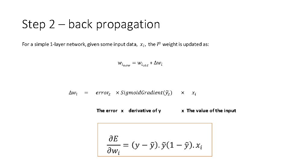
Step 2 – back propagation We will go through the maths of this later on…

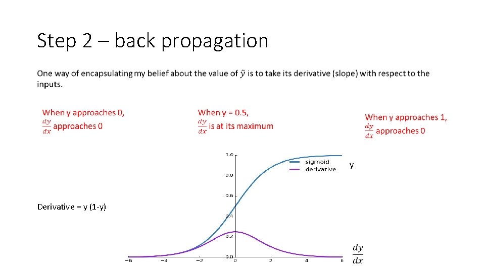
Step 2 – back propagation y Derivative = y (1 -y)

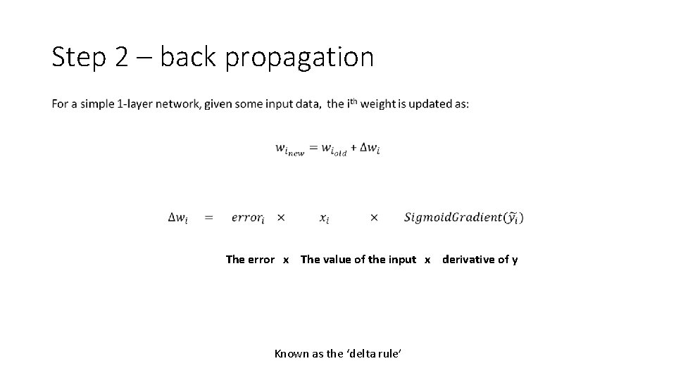
Step 2 – back propagation The error x The value of the input x derivative of y Known as the ‘delta rule’

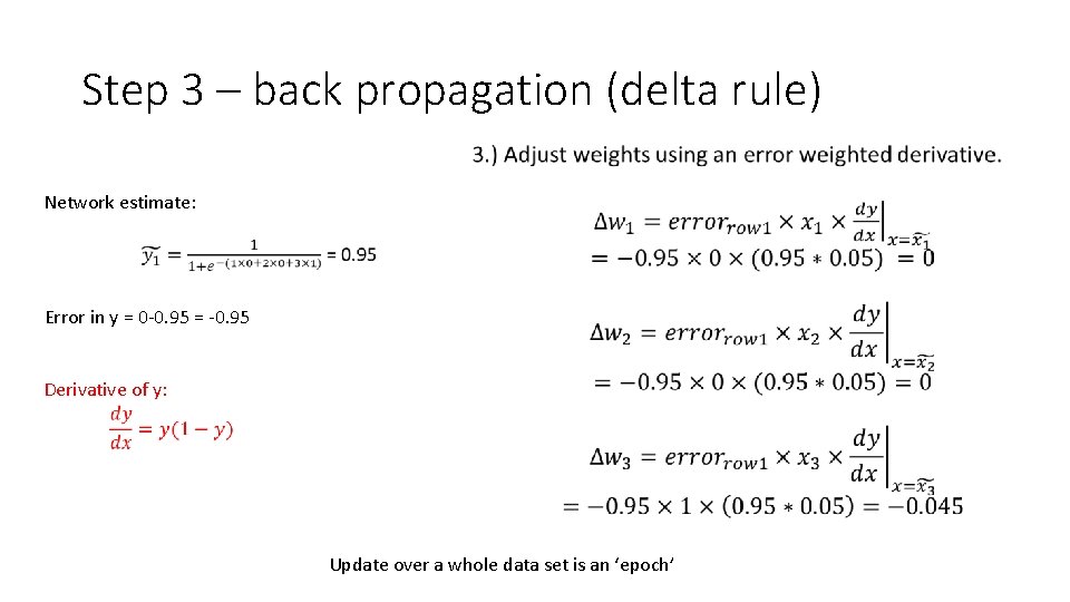
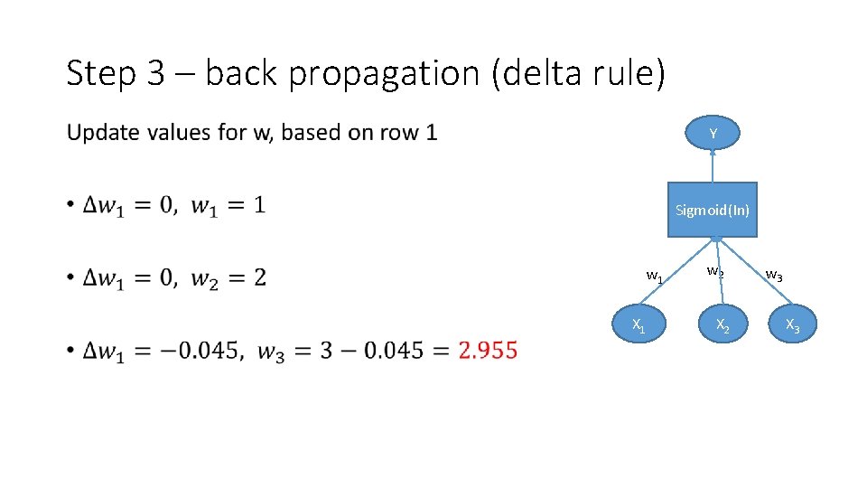
Step 3 – back propagation (delta rule) • Network estimate: Error in y = 0 -0. 95 = -0. 95 Derivative of y: Update over a whole data set is an ‘epoch’

Backpropagation – 1 layer example ØYou will be coding this example, from first-principles, this afternoon. ØTraining Data x 1 x 2 x 3 Y Training row 1 0 0 1 0 Training row 2 1 1 Training row 3 1 0 1 1 Training row 4 0 1 1 0 https: //coderoncode. com/machine/learning/2016/06/06/machine-learning-a-simple-neural-network. html

Step 3 – back propagation (delta rule) • Network estimate: Error in y = 0 -0. 95 = -0. 95 Derivative of y: Update over a whole data set is an ‘epoch’

Step 3 – back propagation (delta rule) • Y Sigmoid(In) w 1 X 1 w 2 X 2 w 3 X 3

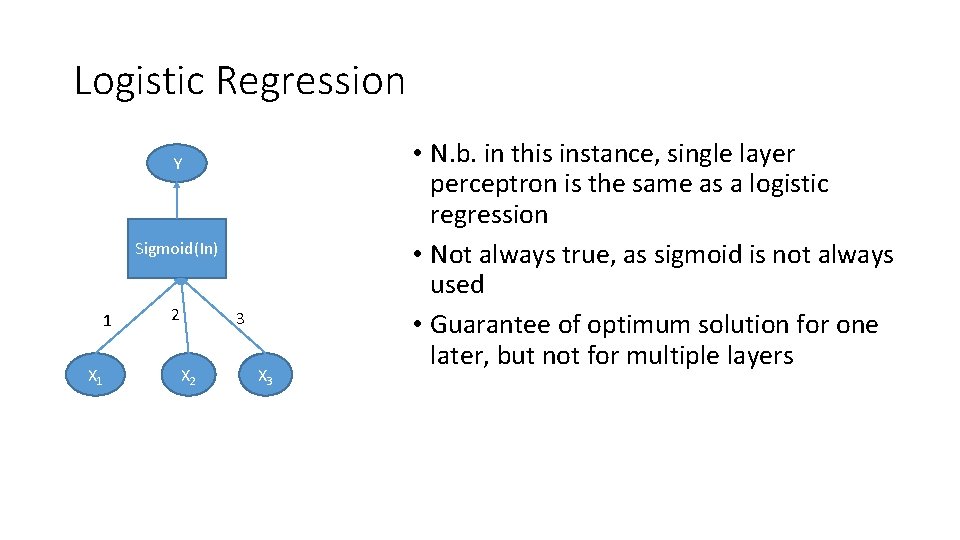
Logistic Regression Y Sigmoid(In) 1 X 1 2 3 X 2 X 3 • N. b. in this instance, single layer perceptron is the same as a logistic regression • Not always true, as sigmoid is not always used • Guarantee of optimum solution for one later, but not for multiple layers

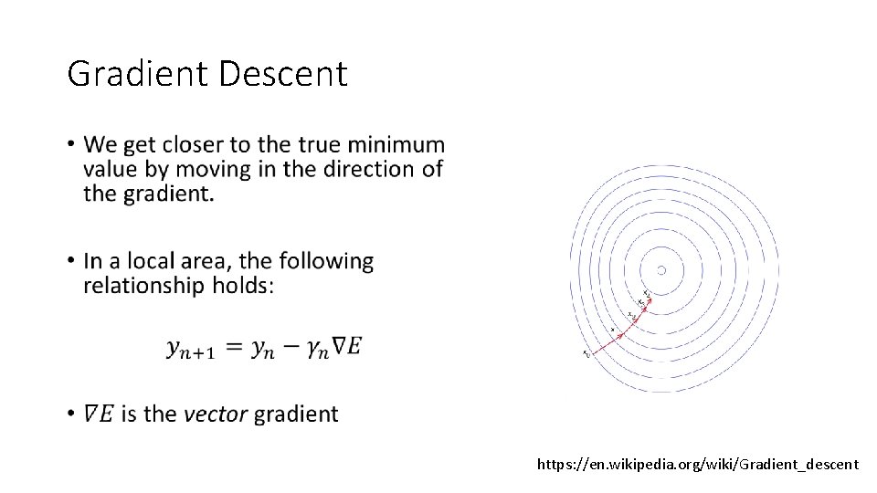
Gradient Descent • https: //en. wikipedia. org/wiki/Gradient_descent

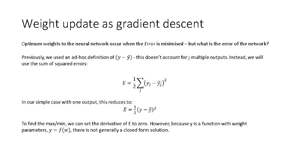
Weight update as gradient descent Optimum weights to the neural network occur when the Error is minimised – but what is the error of the network?

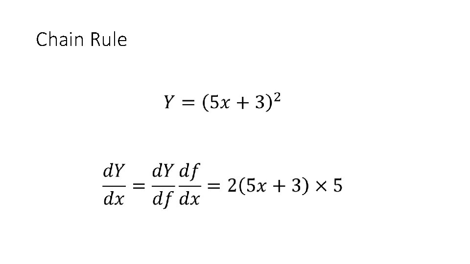
Chain Rule

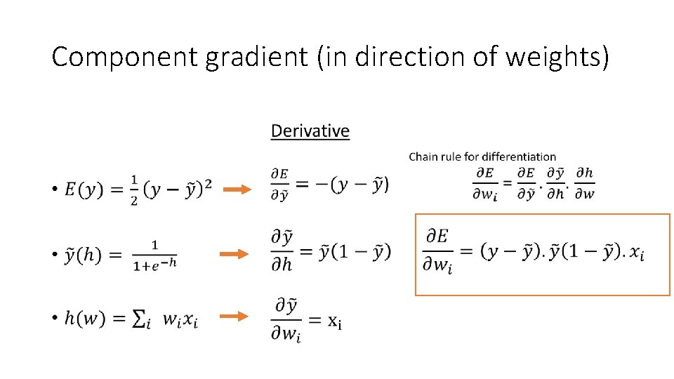
Component gradient (in direction of weights) •

Step 2 – back propagation The error x derivative of y x The value of the input

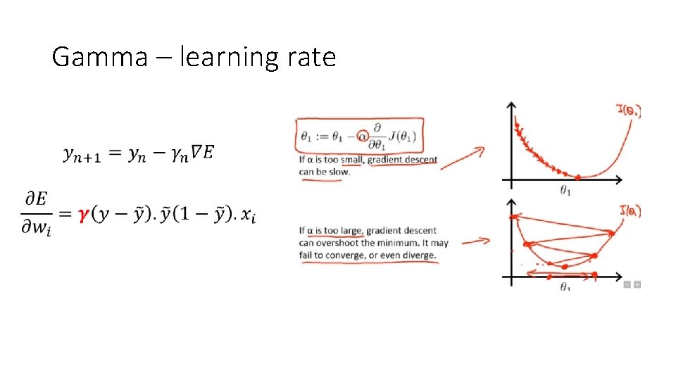
Gamma – learning rate •

Summary so far • Relationship between real and artificial neural networks • Single layer perceptrons (SLPs) • Calculating the input weights for SLPs • Gradient Descent • Limitations of SLPs • Multi-Layer Perceptrons

Break