Introduction to Neural Networks cont Dr David Wong

Introduction to Neural Networks (cont. ) Dr David Wong (With thanks to Dr Gari Clifford, G. I. T)

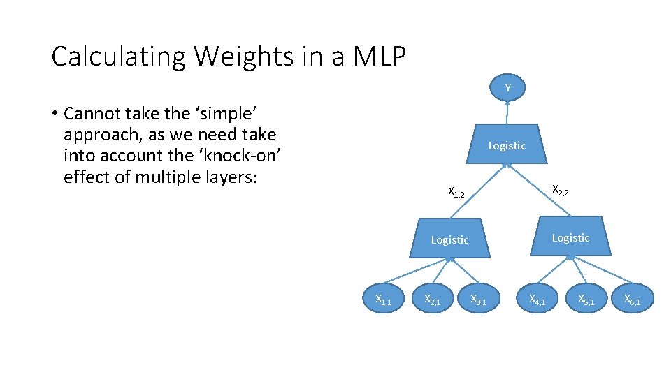
The Multi-Layer Perceptron • single layer can only deal with linearly separable data • Composed of many connected neurons • Three general layers; Input (i), hidden (j) and output (k) • Signals are presented to each input ‘neuron’ or node • Each signal is multiplied by a learned weighting factor (specific to each connection between each layer) • … and by a global activation function, • This is repeated in output layer to map the hidden node values to the output

Calculating Weights in a MLP Y • Cannot take the ‘simple’ approach, as we need take into account the ‘knock-on’ effect of multiple layers: Logistic X 2, 2 X 1, 2 Logistic X 1, 1 X 2, 1 X 3, 1 X 4, 1 X 5, 1 X 6, 1

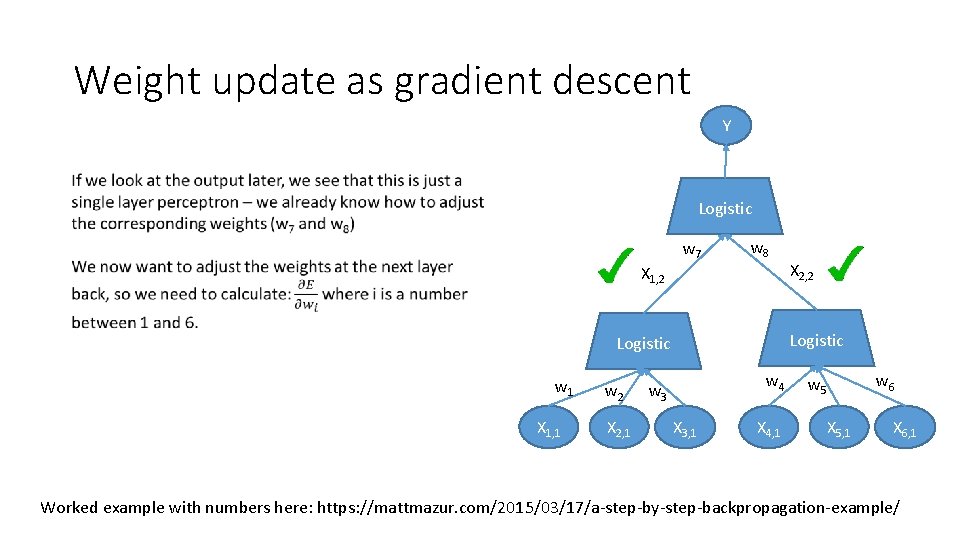
Weight update as gradient descent Y Logistic X 2, 2 X 1, 2 Logistic X 1, 1 X 2, 1 X 3, 1 X 4, 1 X 5, 1 X 6, 1

Weight update as gradient descent Y Logistic w 7 w 8 X 1, 2 Logistic w 1 X 1, 1 w 2 X 2, 1 X 2, 2 w 4 w 3 X 3, 1 X 4, 1 w 6 w 5 X 5, 1 X 6, 1 Worked example with numbers here: https: //mattmazur. com/2015/03/17/a-step-by-step-backpropagation-example/

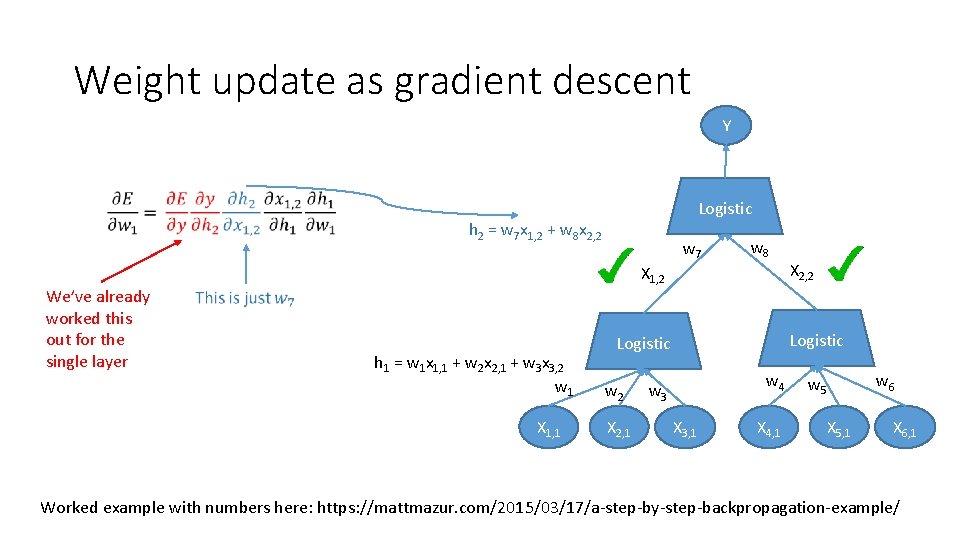
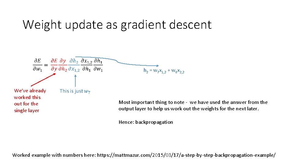
Weight update as gradient descent Y Logistic h 2 = w 7 x 1, 2 + w 8 x 2, 2 We’ve already worked this out for the single layer w 7 w 8 X 1, 2 h 1 = w 1 x 1, 1 + w 2 x 2, 1 + w 3 x 3, 2 w 1 X 1, 1 Logistic w 2 X 2, 1 X 2, 2 w 4 w 3 X 3, 1 X 4, 1 w 6 w 5 X 5, 1 X 6, 1 Worked example with numbers here: https: //mattmazur. com/2015/03/17/a-step-by-step-backpropagation-example/

Weight update as gradient descent h 2 = w 7 x 1, 2 + w 8 x 2, 2 We’ve already worked this out for the single layer Most important thing to note - we have used the answer from the output layer to help us work out the weights for the next later. Hence: backpropagation Worked example with numbers here: https: //mattmazur. com/2015/03/17/a-step-by-step-backpropagation-example/

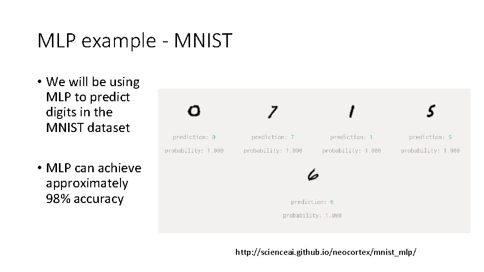
MLP example - MNIST • We will be using MLP to predict digits in the MNIST dataset • MLP can achieve approximately 98% accuracy http: //scienceai. github. io/neocortex/mnist_mlp/

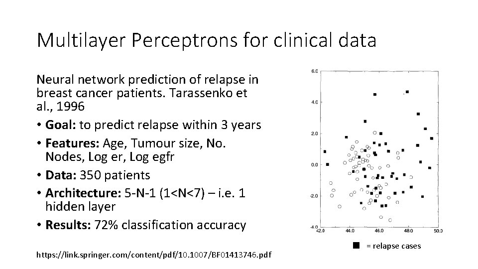
Multilayer Perceptrons for clinical data Neural network prediction of relapse in breast cancer patients. Tarassenko et al. , 1996 • Goal: to predict relapse within 3 years • Features: Age, Tumour size, No. Nodes, Log er, Log egfr • Data: 350 patients • Architecture: 5 -N-1 (1<N<7) – i. e. 1 hidden layer • Results: 72% classification accuracy https: //link. springer. com/content/pdf/10. 1007/BF 01413746. pdf = relapse cases

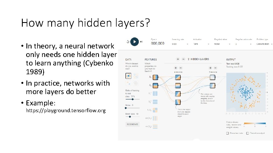
How many hidden layers? • In theory, a neural network only needs one hidden layer to learn anything (Cybenko 1989) • In practice, networks with more layers do better • Example: https: //playground. tensorflow. org

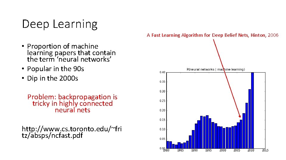
Deep Learning A Fast Learning Algorithm for Deep Belief Nets, Hinton, 2006 • Proportion of machine learning papers that contain the term ‘neural networks’ • Popular in the 90 s • Dip in the 2000 s Problem: backpropagation is tricky in highly connected neural nets http: //www. cs. toronto. edu/~fri tz/absps/ncfast. pdf

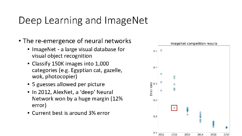
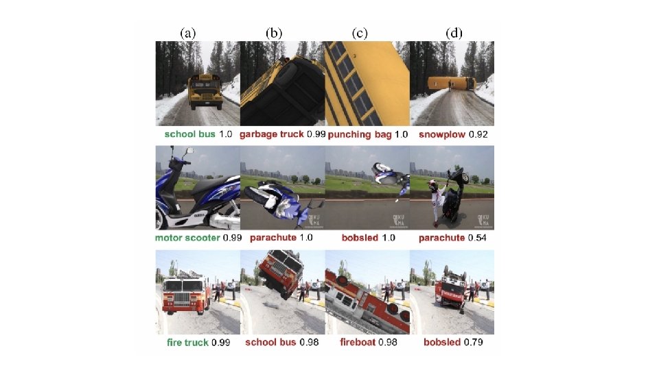
Deep Learning and Image. Net • The re-emergence of neural networks • Image. Net - a large visual database for visual object recognition • Classify 150 K images into 1, 000 categories (e. g. Egyptian cat, gazelle, wok, photocopier) • 5 guesses allowed per picture • In 2012, Alex. Net, a ‘deep’ Neural Network won by a huge margin (12% error) • Current best is around 3% error

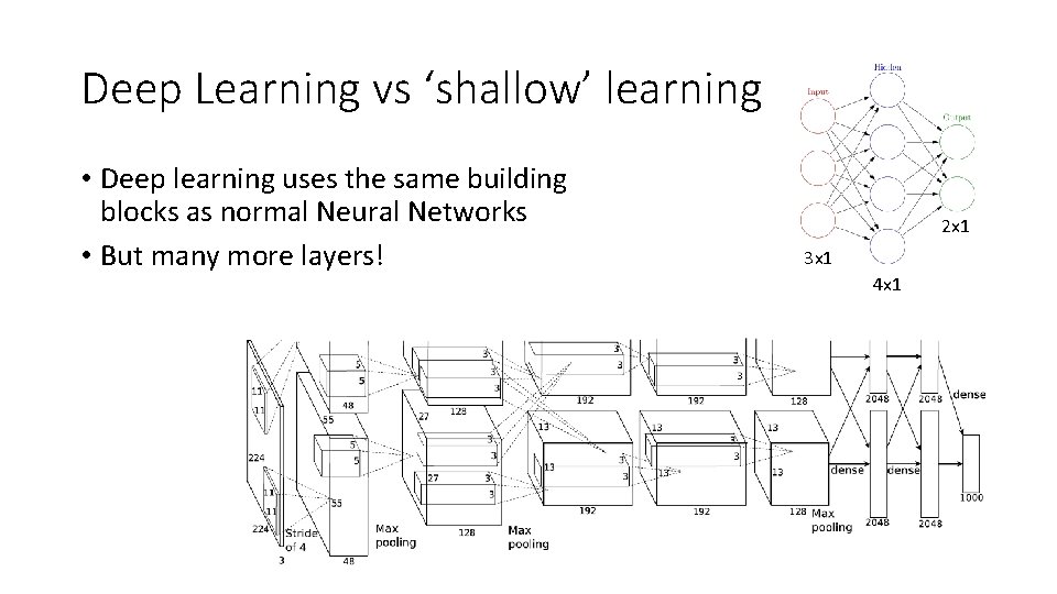
Deep Learning vs ‘shallow’ learning • Deep learning uses the same building blocks as normal Neural Networks • But many more layers! 2 x 1 3 x 1 4 x 1

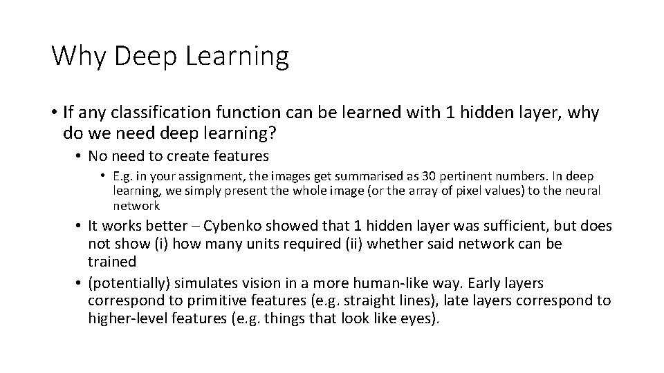
Why Deep Learning • If any classification function can be learned with 1 hidden layer, why do we need deep learning?

Why Deep Learning • If any classification function can be learned with 1 hidden layer, why do we need deep learning? • No need to create features • E. g. in your assignment, the images get summarised as 30 pertinent numbers. In deep learning, we simply present the whole image (or the array of pixel values) to the neural network • It works better – Cybenko showed that 1 hidden layer was sufficient, but does not show (i) how many units required (ii) whether said network can be trained • (potentially) simulates vision in a more human-like way. Early layers correspond to primitive features (e. g. straight lines), late layers correspond to higher-level features (e. g. things that look like eyes).

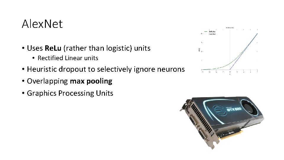
Alex. Net • Uses Re. Lu (rather than logistic) units • Rectified Linear units • Heuristic dropout to selectively ignore neurons • Overlapping max pooling • Graphics Processing Units

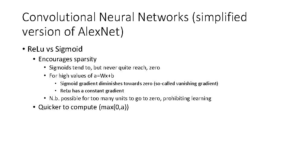
Convolutional Neural Networks (simplified version of Alex. Net) • Re. Lu vs Sigmoid • Encourages sparsity • Sigmoids tend to, but never quite reach, zero • For high values of a=Wx+b • Sigmoid gradient diminishes towards zero (so-called vanishing gradient) • Re. Lu has a constant gradient • N. b. possible for too many units to go to zero, prohibiting learning • Quicker to compute (max(0, a))

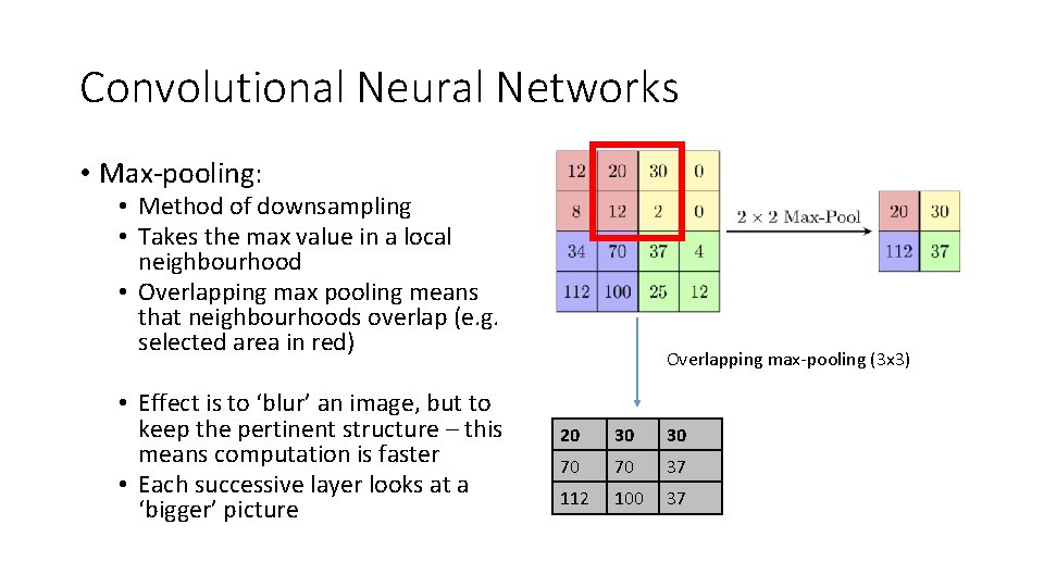
Convolutional Neural Networks • Max-pooling: • Method of downsampling • Takes the max value in a local neighbourhood • Overlapping max pooling means that neighbourhoods overlap (e. g. selected area in red) • Effect is to ‘blur’ an image, but to keep the pertinent structure – this means computation is faster • Each successive layer looks at a ‘bigger’ picture Overlapping max-pooling (3 x 3) 20 30 30 70 70 37 112 100 37

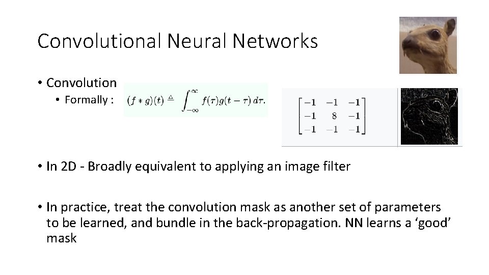
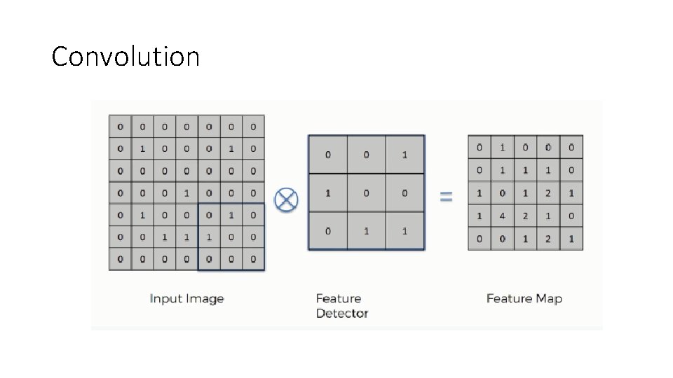
Convolutional Neural Networks • Convolution • Formally : • In 2 D - Broadly equivalent to applying an image filter • In practice, treat the convolution mask as another set of parameters to be learned, and bundle in the back-propagation. NN learns a ‘good’ mask

Convolution

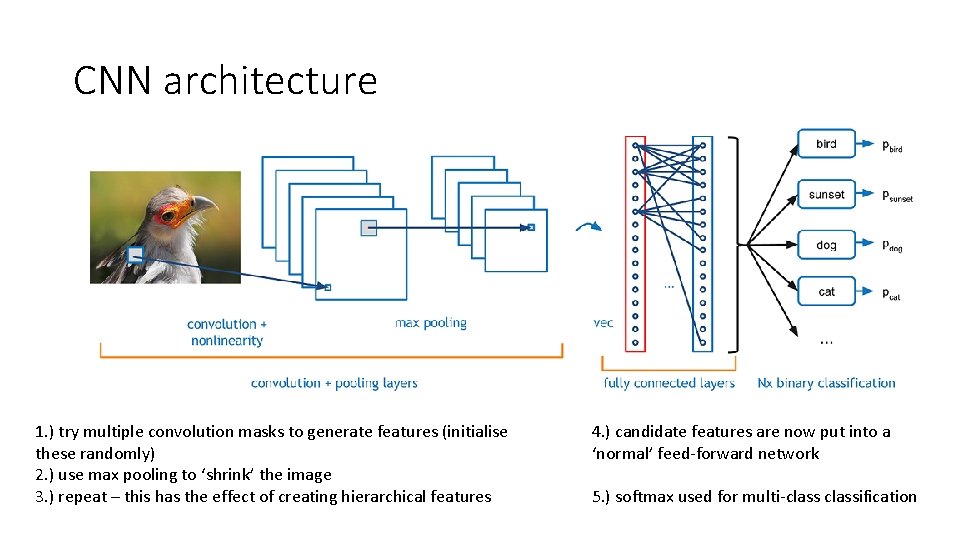
CNN architecture 1. ) try multiple convolution masks to generate features (initialise these randomly) 2. ) use max pooling to ‘shrink’ the image 3. ) repeat – this has the effect of creating hierarchical features 4. ) candidate features are now put into a ‘normal’ feed-forward network 5. ) softmax used for multi-classification

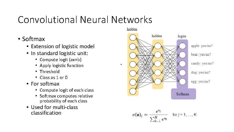
Convolutional Neural Networks • Softmax • Extension of logistic model • In standard logistic unit: • • Compute logit (ax+b) Apply logistic function Threshold Class as 1 or 0 • For softmax • Compute logit of each class • Softmax computes relative probability of each class • Used for multi-classification

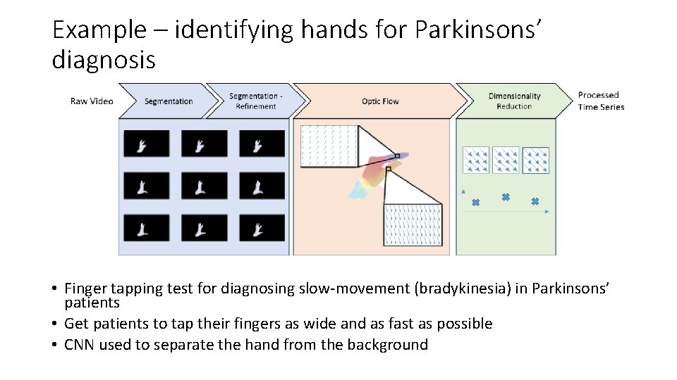
Example – identifying hands for Parkinsons’ diagnosis • Finger tapping test for diagnosing slow-movement (bradykinesia) in Parkinsons’ patients • Get patients to tap their fingers as wide and as fast as possible • CNN used to separate the hand from the background

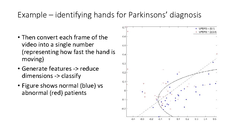
Example – identifying hands for Parkinsons’ diagnosis • Then convert each frame of the video into a single number (representing how fast the hand is moving) • Generate features -> reduce dimensions -> classify • Figure shows normal (blue) vs abnormal (red) patients

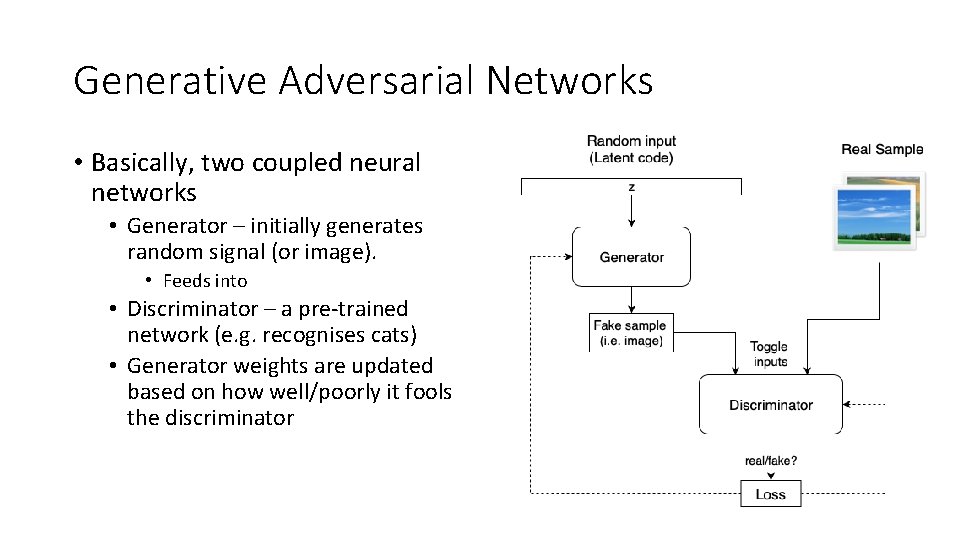
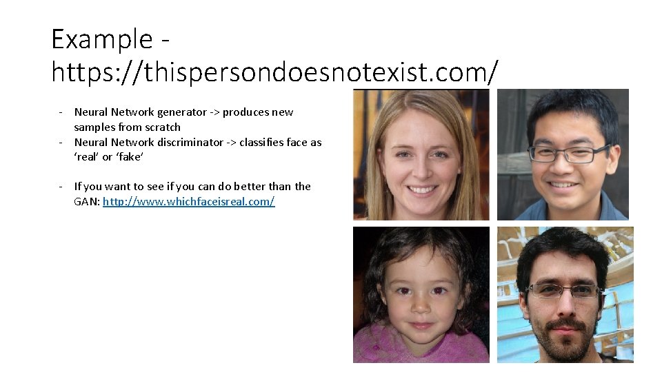
Generative Adversarial Networks • Basically, two coupled neural networks • Generator – initially generates random signal (or image). • Feeds into • Discriminator – a pre-trained network (e. g. recognises cats) • Generator weights are updated based on how well/poorly it fools the discriminator

Example https: //thispersondoesnotexist. com/ - Neural Network generator -> produces new samples from scratch - Neural Network discriminator -> classifies face as ‘real’ or ‘fake’ - If you want to see if you can do better than the GAN: http: //www. whichfaceisreal. com/