INTRODUCTION TO NEURAL NETWORKS AND LEARNING What is

INTRODUCTION TO NEURAL NETWORKS AND LEARNING

What is Neural Network? Computational model inspired by biological Neuron, cells perform information processing in brain Systems are trained rather than programmed to accomplish tasks Successful at solving problems proven difficult or impossible by using conventional computing techniques * Formal Definition : A Neural Network is a non-programmed adaptive information processing system based upon research in how the brain encodes and processes information

Biological Neuron Excerpted from Artificial Intelligence: Modern Approach by S. Russel and P. Norvig

Properties of Biological Neuron and Brain Neurotransmission by means of electrical impulse effected by chemical transmitter Period of latent summation generate impulse if total potential of membrane reaches a level : firing excitatory - inhibitory Human Brain Cerebral cortex Areas of Brain for specific function 1011 neurons 104 synapses per neuron 10 -3 sec cycle time (computer : 10 -8 sec)

Computational Model of a Neuron SOMA T Dendrites (input) Summer synapses Threshold 1 0 Axons (output)

What Makes Up a Neural Network? Neural Net Neurobiology Processing Element Neuron Interconnections Scheme Dendrites and Axons Learning Law Neuro Transmitters

Neural Net vs. Von Neumann Computer Neural Net Von Neumann Non-algorithmic Algorithmic Trained Programmed with instructions Memory and processing elements the same Memory and processing separate Pursue multiple hypotheses simultaneously Pursue one hypothesis at a time Fault tolerant Non fault tolerant Non-logical operation Highly logical operation Adaptation or learning Algorithmic parameterization modification only Seeks answer by finding minima in solution space Seeks answer by following logical tree structure

What is Learning ? Concepts of inductive learning (learning from example) Example : (x, f(x)) Inductive inference Hypothesis : h [collection of examples of (x, f(X))] h(X) approximation of f, the agent’s belief about f ( h f ) hypothesis space : set of all hypothesis writable. Bias Any preference for one hypothesis over anothere’re many consistent hypotheses.

Examples of biased hypothesis (a) examples (b) hypothesis 1 (c) hypothesis 2 (d) hypothesis 3 Representation of functions expressiveness : perceptron can’t learn XOR efficiency : # of examples for good generalization ‘a good set of sentences’

Learning Procedure 1. 2. 3. 4. 5. Collect a large set of examples Divide it into two disjoint sets : training set & test set Use the learning algorithm with the training set as examples to generate a hypothesis H Measure the percentage of examples in the test set that are correctly classified by H. Repeat steps 1 -4 for different sizes of training sets & different randomly selected training sets of each size

SINGLE THRESHOLD LOGIC UNIT(TLU)

Introduction : S-R Learning with TLU/NN Experiences sensory data set paired with proper action Knowledge function from sensory data to proper action Representation 1. single TLU with adjustable weights 2. Multi layer perceptron

Training Single TLU geometry TLU definition internal knowledge representation an abstract computation tool that calculates Input : output : transfer : weight : threshold : 1 0

Geometric Interpretation of TLU computation 0 if X is in one side of a hyperplane, 1 if X is in the other side of the hyperplane. A hyper plane in Rn space:

Training Single TLU : Gradient Descent Method Definition Gradient Descent Methods Learning is a search over internal representations, which maximize/minizie some evaluation function : TLU output : desired output : ε can be minimized by gradient descent : greedy method How to update W? ? Incremental learning : adjust W that slightly reduce e for one Xi Batch learning : adjust W that reduce e for all Xi

– Gradient descent learning rule (Single TLU, Incremental) Gradient by Definition By Chainrule case 1) case 2)

Training Single TLU : Widrow-Hoff Procedure Activation function:

Training Single TLU : Generalized Delta Activation function: Sigmoid function

Training Single TLU : Error Correction Procedure Learning rule Activation function : 0/1 threshold function Adjust weights, only when (d-f) = (1 or -1) Use the same weight update gradient 1 0 Termination of Learning Procedure Error Correction Procedure If there exists some weight vector W, that produces a correct output for all input vectors, the error-correction procedure will find such a weight vector and terminate. If there exists no such vector W, error-correction procedure will never terminate. Widrow-hoff and Generalized Delta procedures Minimum squared-error solutions are found even when there exist no perfect solutions W.

– Example problem 0/1 situations are linearly separable! Home work !!

NEURAL NETWORKS

Neural Networks Why Neural Networks? A single TLU is not enough ! There are sets of stimuli and responses that cannot be learned by a single TLU. (non linearly separable functions) Let’s use a network of TLUs ! Structure of Neural Networks Feed forward net: There is no circuit in the net, output value is dependent on only input values. Recurrent net : There are circuits in the net, output value is dependent on input & history.

An Example of a Neural Network 3 layer feed forward network Input layer Hidden layer Output layer

Neural Network: Notations j-th Layer output vector : Input vector Final layer output vector : Weight vector of i-th TLU in j-th layer Input to a i-th TLU in j-th layer (activation) : Number of TLUs in j-th layer :

A general, k-layer feed forward network

Backpropagation Method(1/3) Gradient of squared error with respect to weight vector Using activation variable and the chain rule Let activation error influence Weight update rule is derived:

Backpropagation Method(2/3) Weight update rule in final layer By definition Since f is the sigmoid function of Backpropagation weight adjustment rule for the single TLU in the final layer:

Backpropagation Method(3/3) Weight update rule in intermediate layers Using chain rule

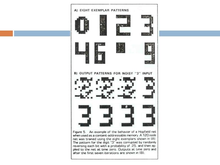
Recurrent Neural Networks : Hopfield Network Proper when exact binary representations are possible. Can be used as an associative memory or to solve optimization problems. The number of classes (M) must be kept smaller than 0. 15 times the number of nodes (N).

OUTPUTS(Valid After Convergence) x’ 0 x’ 1 x’N-2 x’N-1 . . . x 0 x 1 x. N-2 INPUTS(Applied At Time Zero) x. N-1

Recurrent Neural Networks : Hopfield Network Algorithm(1/2) Step 1 : Assign Connection Weights. Step 2 : Initialize with unknown input pattern.

Recurrent Neural Networks : Hopfield Network Algorithm (2/2) Step 3 : Iterate until convergence. 1 0 -1 Step 4 : goto step 2.

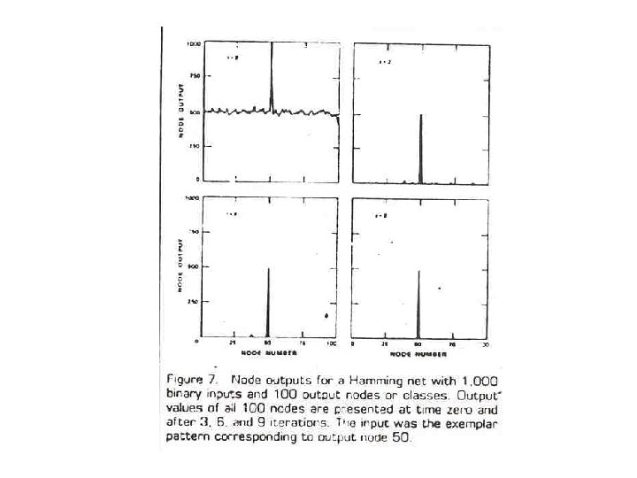
Recurrent Neural Networks : Hamming Net Optimum minimum error classifier Calculate Hamming distance to the exemplar for each class and selects that class with minimum Hamming distance = number of different bits Advantages Over Hopfield Net: Hopfield Net is worse than or equivalent to Hamming Net requires fewer connections The number of connections in Hamming Net grows linearly N=100, M=10 N 2 vs 10000 NM + M 2 → M(N+M) 1100 ≈ NM (1000) N >> M

OUTPUT(valid after MAXNET converge) Y 0 Y 1 YM-2 YM-1 (Class) MAXNET PICKS MAXIMUM Tkl CALCULATE MATCHING SCORES Wij x 0 x 1 x. N-2 x. N-1 INPUT(applied at time zero) (Data)

Recurrent Neural Networks : Hamming Net Algorithm Step 1. Assign Connection Weights and offsets in the lower subnet : in the upper subnet : for lateral inhibition

Step 2. Initialize with unknown input pattern Step 3. Iterate until convergence f t: 1 This process is repeated until convergence. Step 4. Go to step 2 1

Self Organizing Feature Map Transform input patterns of arbitrary dimension to discrete map of lower dimension clustering representation by representative Algorithm 1. initialize w’s 2. find nearest cell i(x) = argminj || x(n) - wj(n) || 3. update weights of i(x) and its neighbors wj(n+1) = wj(n) + (n) [ x(n) - wj(n) ] 4. reduce neighbors and 5. Go to 2 x 1 x 2 NE(n) j NE(n+1)

SOFM Example Input sample : random numbers within 2 -D unit square 100 neurons ( 10 x 10) Initial weights : random assignment (0. 0~1. 0) Display each neuron positioned at w 1, w 2 neighbors are connected by line

Input samples Initial weights

After 25 iterations After 10000 iterations Programming Assignment!!