Introduction to Neural Networks 1 Overview 1 The

Introduction to Neural Networks 1

Overview 1. The motivation for NNs 2. Neuron – The basic unit 3. Fully-connected Neural Networks A. Feedforward (inference) B. The linear algebra behind 4. Convolutional Neural Networks & Deep Learning 2

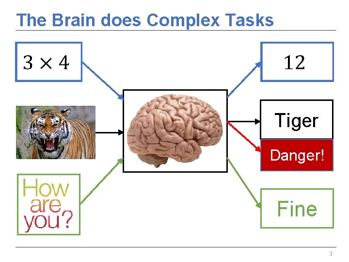
The Brain does Complex Tasks Tiger Danger! Fine 3

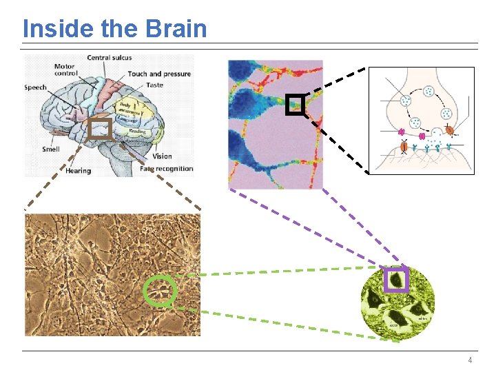
Inside the Brain 4

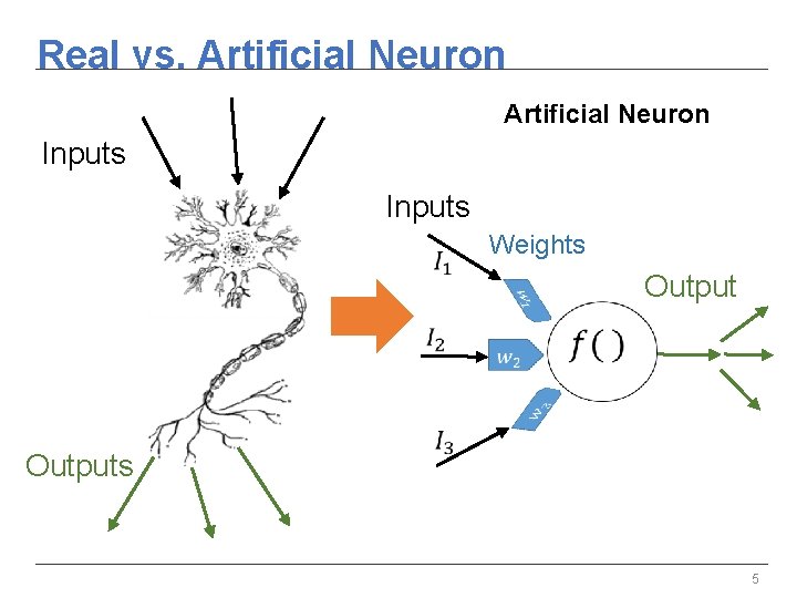
Real vs. Artificial Neuron Inputs Weights Output Outputs 5

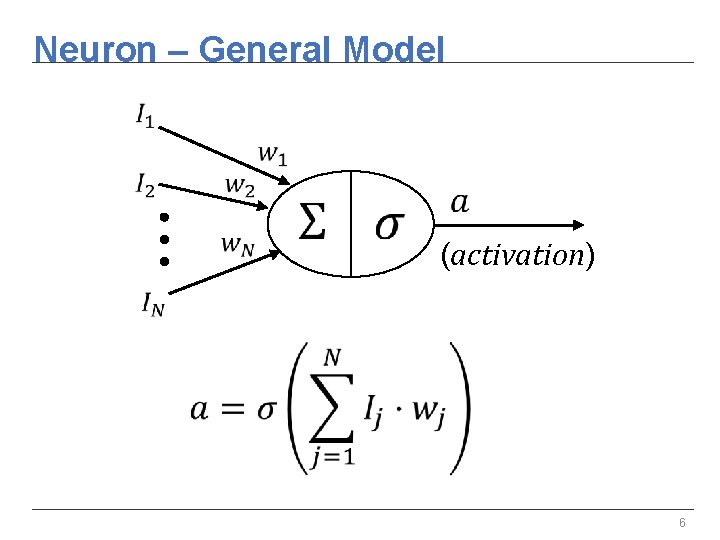
Neuron – General Model (activation) 6

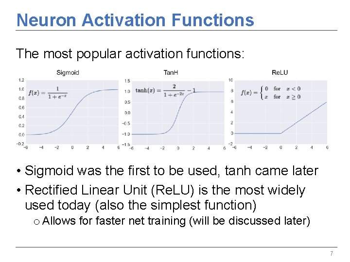
Neuron Activation Functions The most popular activation functions: • Sigmoid was the first to be used, tanh came later • Rectified Linear Unit (Re. LU) is the most widely used today (also the simplest function) o Allows for faster net training (will be discussed later) 7

Overview ü The motivation for NNs ü Neuron – The basic unit 3. Fully-connected Neural Networks A. Feedforward (inference) B. The linear algebra behind 4. Convolutional Neural Networks & Deep Learning 8

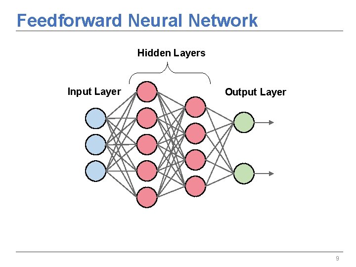
Feedforward Neural Network Hidden Layers Input Layer Output Layer 9

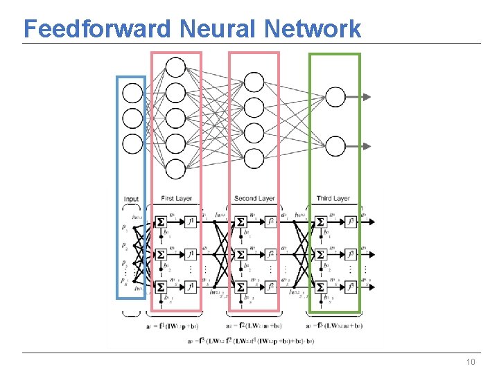
Feedforward Neural Network 10

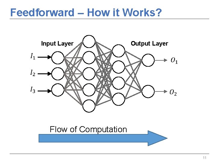
Feedforward – How it Works? Input Layer Output Layer Flow of Computation 11

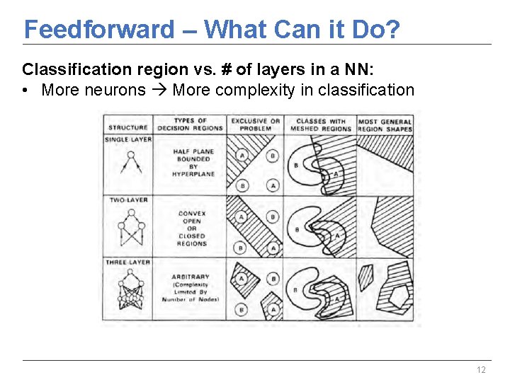
Feedforward – What Can it Do? Classification region vs. # of layers in a NN: • More neurons More complexity in classification 12

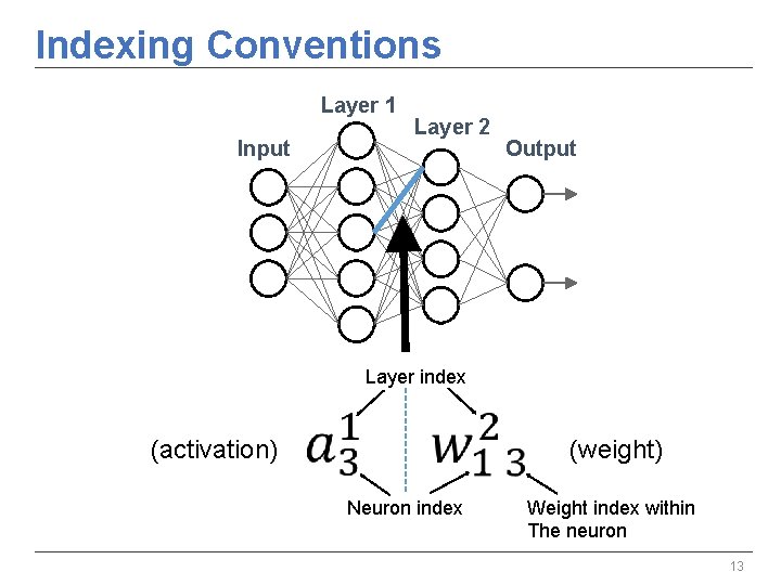
Indexing Conventions Layer 1 Input Layer 2 Output Layer index (weight) (activation) Neuron index Weight index within The neuron 13

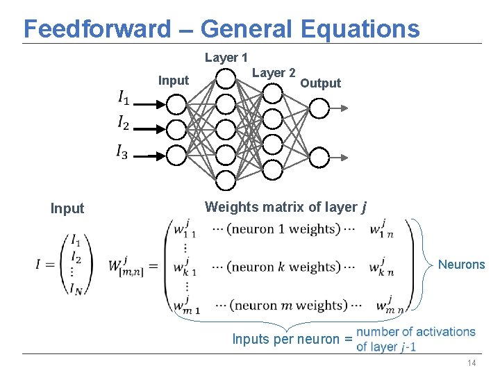
Feedforward – General Equations Layer 1 Input Layer 2 Output Weights matrix of layer j Input Neurons Inputs per neuron = 14

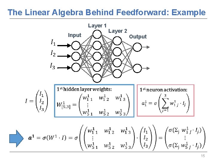
The Linear Algebra Behind Feedforward: Example Layer 1 Input Layer 2 Output 15

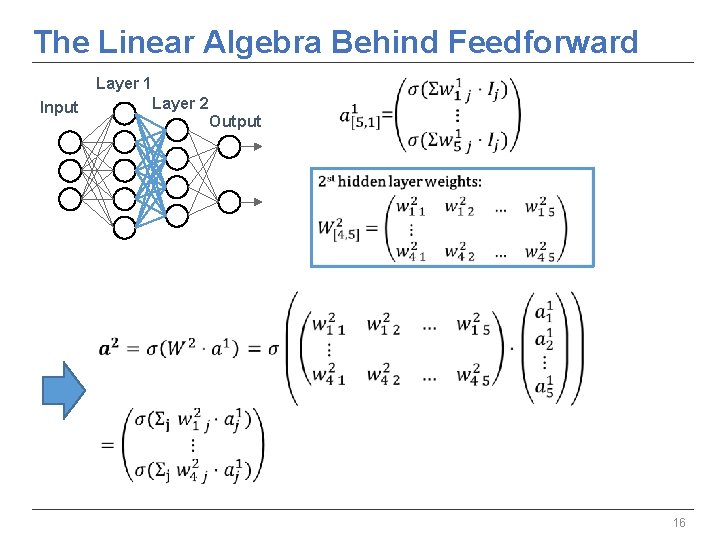
The Linear Algebra Behind Feedforward Layer 1 Layer 2 Input Output 16

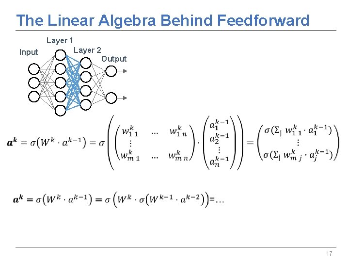
The Linear Algebra Behind Feedforward Layer 1 Input Layer 2 Output 17

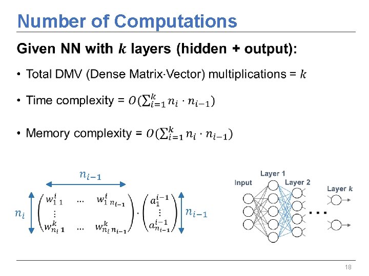
Number of Computations • 18

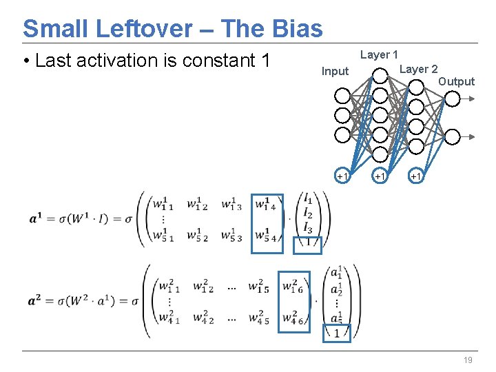
Small Leftover – The Bias • Last activation is constant 1 Layer 2 Input +1 Output +1 +1 19

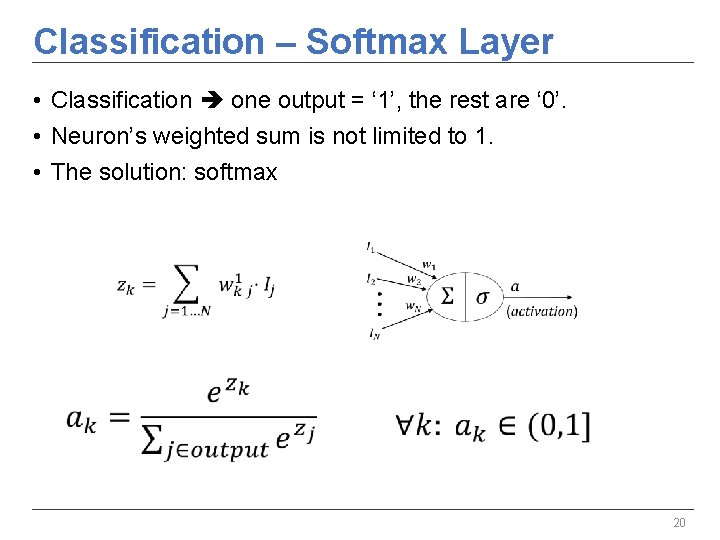
Classification – Softmax Layer • Classification one output = ‘ 1’, the rest are ‘ 0’. • Neuron’s weighted sum is not limited to 1. • The solution: softmax 20

Overview ü The motivation for NNs ü Neuron – The basic unit ü Fully-connected Neural Networks A. Feedforward (inference) B. The linear algebra behind 4. Convolutional Neural Networks & Deep Learning 21

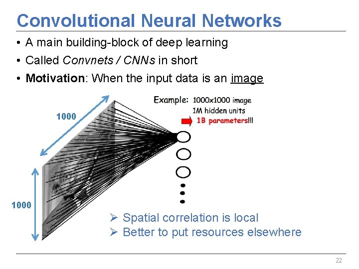
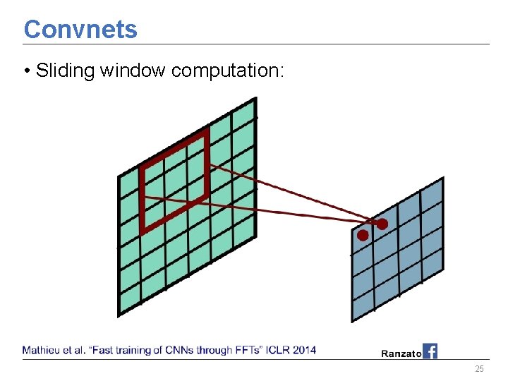
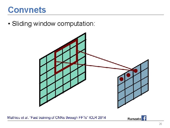
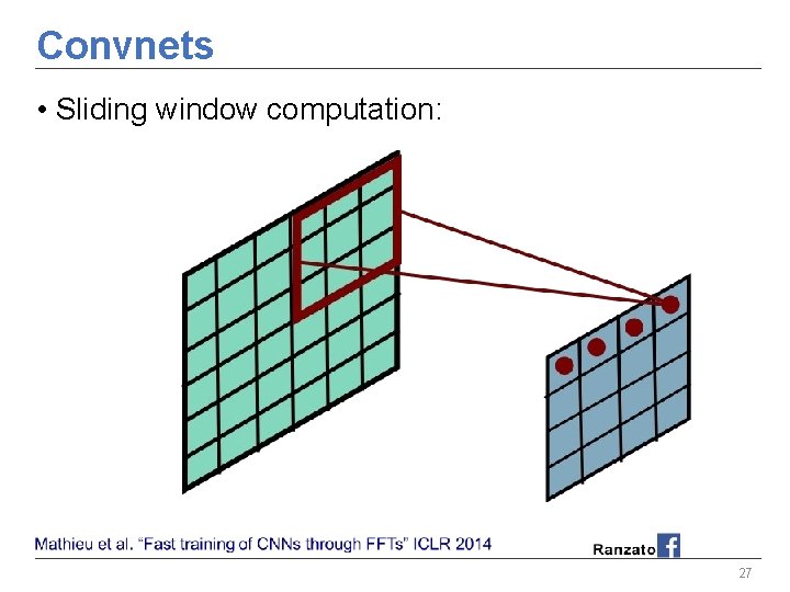
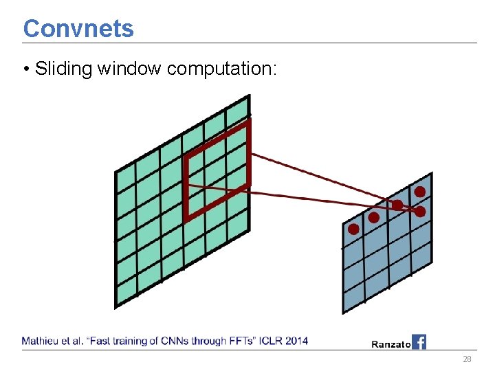
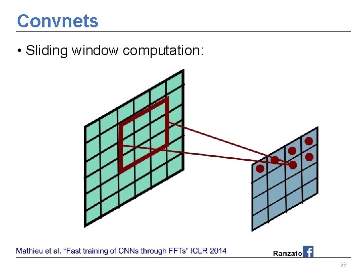
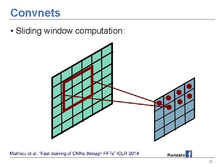
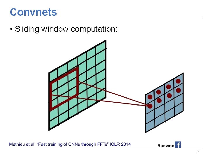
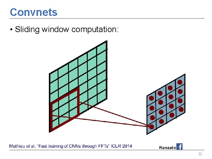
Convolutional Neural Networks • A main building-block of deep learning • Called Convnets / CNNs in short • Motivation: When the input data is an image 1000 Ø Spatial correlation is local Ø Better to put resources elsewhere 22

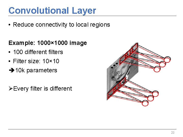
Convolutional Layer • Reduce connectivity to local regions Example: 1000× 1000 image • 100 different filters • Filter size: 10× 10 10 k parameters ØEvery filter is different 23

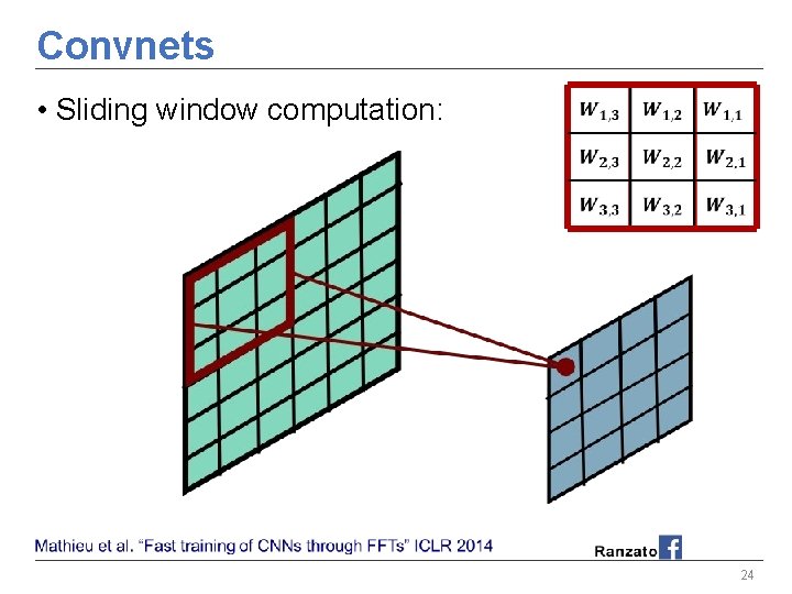
Convnets • Sliding window computation: 24

Convnets • Sliding window computation: 25

Convnets • Sliding window computation: 26

Convnets • Sliding window computation: 27

Convnets • Sliding window computation: 28

Convnets • Sliding window computation: 29

Convnets • Sliding window computation: 30

Convnets • Sliding window computation: 31

Convnets • Sliding window computation: 32

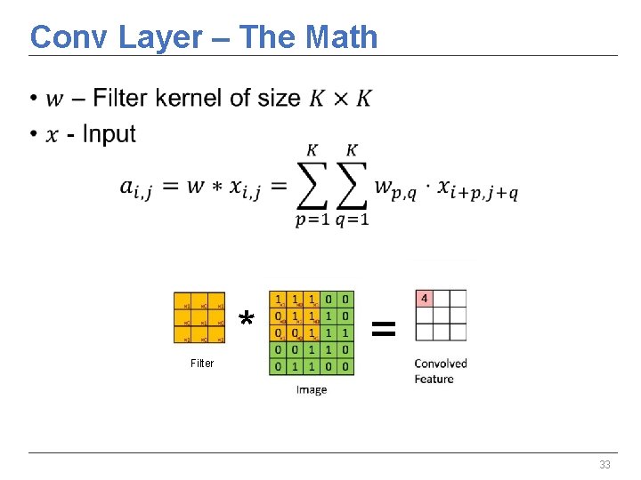
Conv Layer – The Math • * = Filter 33

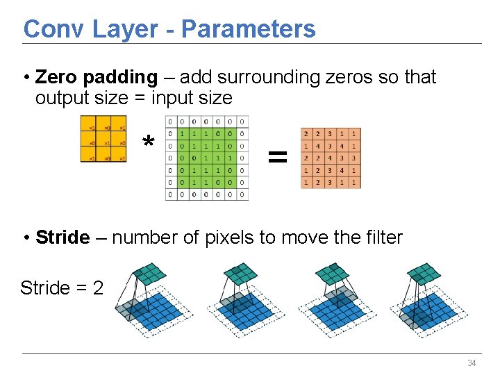
Conv Layer - Parameters • Zero padding – add surrounding zeros so that output size = input size * = • Stride – number of pixels to move the filter Stride = 2 34

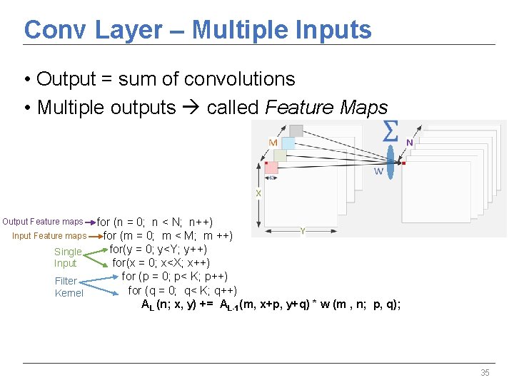
Conv Layer – Multiple Inputs • Output = sum of convolutions • Multiple outputs called Feature Maps Output Feature maps Input Feature maps Single Input Filter Kernel for (n = 0; n < N; n++) for (m = 0; m < M; m ++) for(y = 0; y<Y; y++) for(x = 0; x<X; x++) for (p = 0; p< K; p++) for (q = 0; q< K; q++) AL (n; x, y) += AL-1(m, x+p, y+q) * w (m , n; p, q); 35

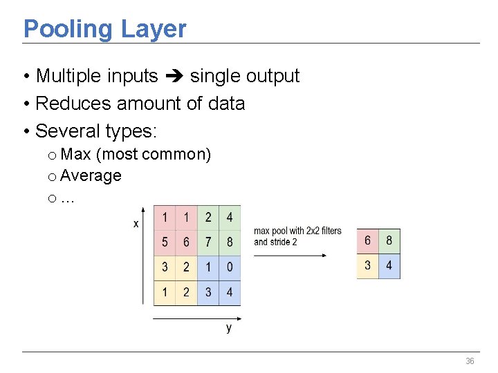
Pooling Layer • Multiple inputs single output • Reduces amount of data • Several types: o Max (most common) o Average o… 36

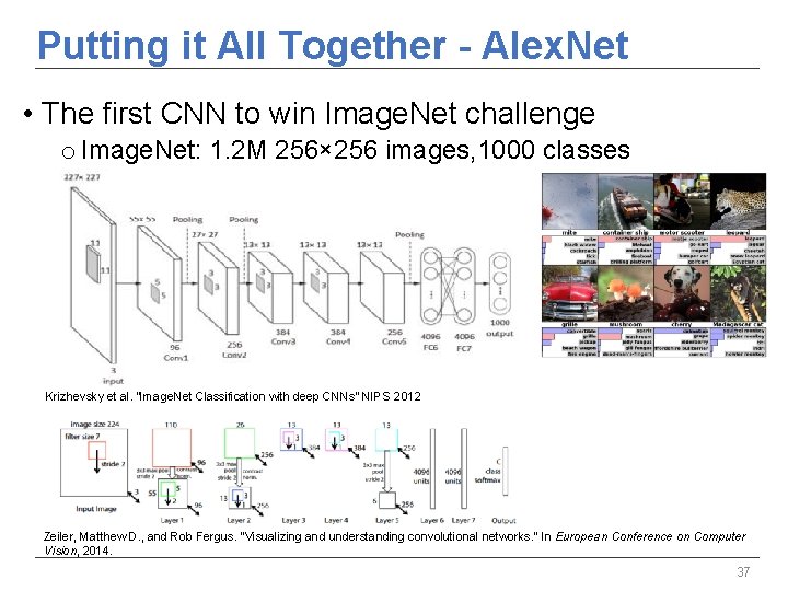
Putting it All Together - Alex. Net • The first CNN to win Image. Net challenge o Image. Net: 1. 2 M 256× 256 images, 1000 classes Krizhevsky et al. “Image. Net Classification with deep CNNs” NIPS 2012 Zeiler, Matthew D. , and Rob Fergus. "Visualizing and understanding convolutional networks. " In European Conference on Computer Vision, 2014. 37

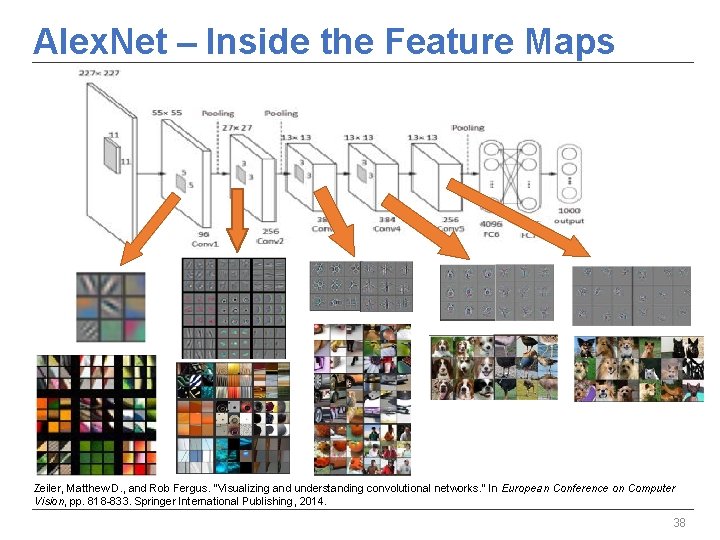
Alex. Net – Inside the Feature Maps Zeiler, Matthew D. , and Rob Fergus. "Visualizing and understanding convolutional networks. " In European Conference on Computer Vision, pp. 818 -833. Springer International Publishing, 2014. 38

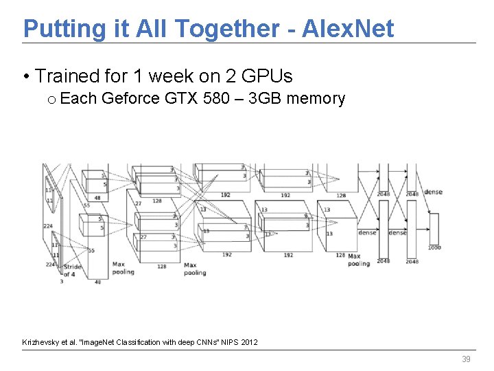
Putting it All Together - Alex. Net • Trained for 1 week on 2 GPUs o Each Geforce GTX 580 – 3 GB memory Krizhevsky et al. “Image. Net Classification with deep CNNs” NIPS 2012 39

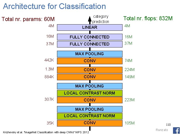
Architecture for Classification 4 M category prediction LINEAR 16 M FULLY CONNECTED 16 M 37 M FULLY CONNECTED 37 M Total nr. params: 60 M Total nr. flops: 832 M 4 M MAX POOLING 442 K CONV 74 M 1. 3 M CONV 224 M 884 K CONV 149 M MAX POOLING LOCAL CONTRAST NORM 307 K CONV 223 M MAX POOLING LOCAL CONTRAST NORM 35 K CONV Krizhevsky et al. “Image. Net Classification with deep CNNs” NIPS 2012 105 M 110 Ranzato

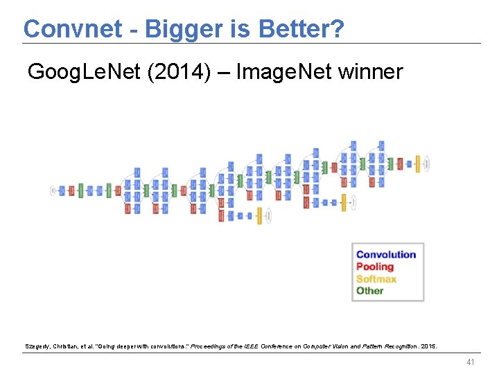
Convnet - Bigger is Better? Goog. Le. Net (2014) – Image. Net winner Szegedy, Christian, et al. "Going deeper with convolutions. " Proceedings of the IEEE Conference on Computer Vision and Pattern Recognition. 2015. 41

Thank you 42