Introduction to Mixed Effects and Repeated Measures Models

- Slides: 70

Introduction* to Mixed Effects and Repeated Measures Models Presented by Peter Westfall, Professor of Statistics, Texas Tech Warning: There will be a quiz *Some material is adapted from Brown and Prescott, Applied Mixed Models in Medicine, Wiley New York (1999); Some from Littell et al. The SAS System For Mixed Models, SAS Institute Inc. 1996 1

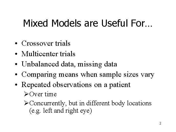
Mixed Models are Useful For… • • • Crossover trials Multicenter trials Unbalanced data, missing data Comparing means when sample sizes vary Repeated observations on a patient ØOver time ØConcurrently, but in different body locations (e. g. left and right eye) 2

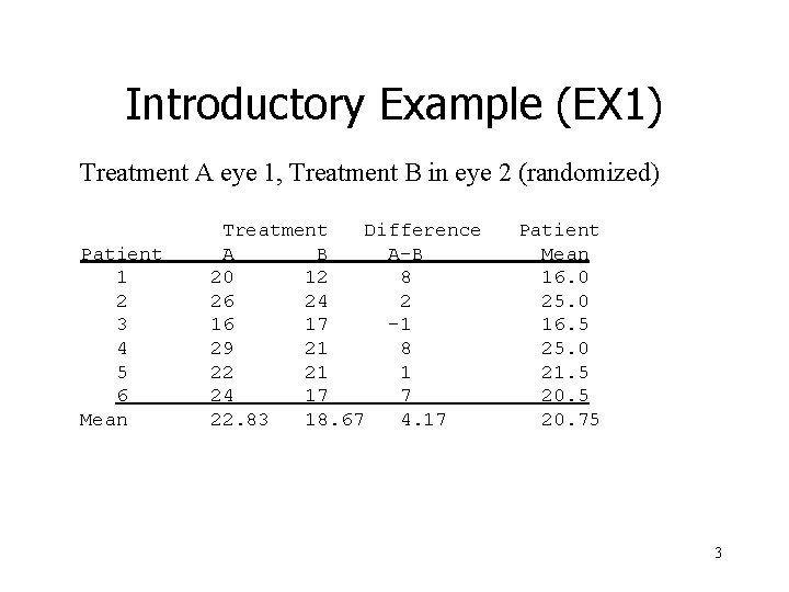
Introductory Example (EX 1) Treatment A eye 1, Treatment B in eye 2 (randomized) Patient 1 2 3 4 5 6 Mean Treatment Difference A B A-B 20 12 8 26 24 2 16 17 -1 29 21 8 22 21 1 24 17 7 22. 83 18. 67 4. 17 Patient Mean 16. 0 25. 0 16. 5 25. 0 21. 5 20. 75 3

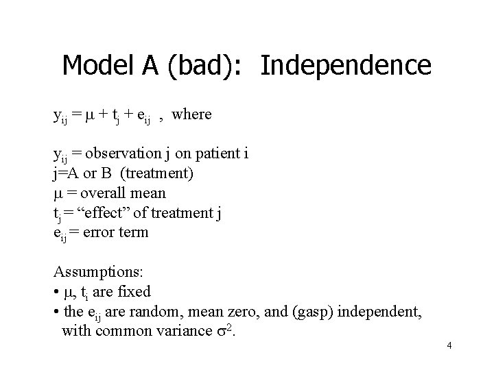
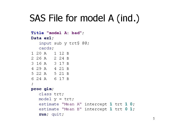
Model A (bad): Independence yij = m + tj + eij , where yij = observation j on patient i j=A or B (treatment) m = overall mean tj = “effect” of treatment j eij = error term Assumptions: • m, ti are fixed • the eij are random, mean zero, and (gasp) independent, with common variance s 2. 4

SAS File for model A (ind. ) Title "model A: bad"; Data ex 1; input sub y trt$ @@; cards; 1 20 A 1 12 B 2 26 A 2 24 B 3 16 A 3 17 B 4 29 A 4 21 B 5 22 A 5 21 B 6 24 A 6 17 B ; proc glm; class trt; model y = trt; estimate "Mean A" intercept 1 trt 1 0; estimate "Mean B" intercept 1 trt 0 1; run; quit; 5

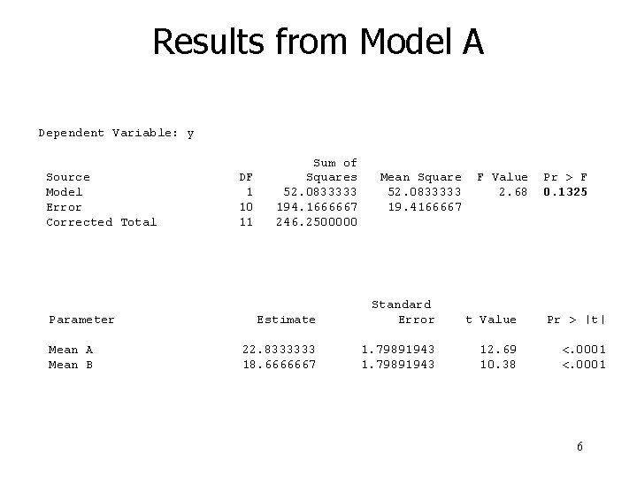
Results from Model A Dependent Variable: y Source Model Error Corrected Total Parameter Mean A Mean B DF 1 10 11 Sum of Squares 52. 0833333 194. 1666667 246. 2500000 Mean Square 52. 0833333 19. 4166667 F Value 2. 68 Pr > F 0. 1325 Estimate Standard Error t Value Pr > |t| 22. 8333333 18. 6666667 1. 79891943 12. 69 10. 38 <. 0001 6

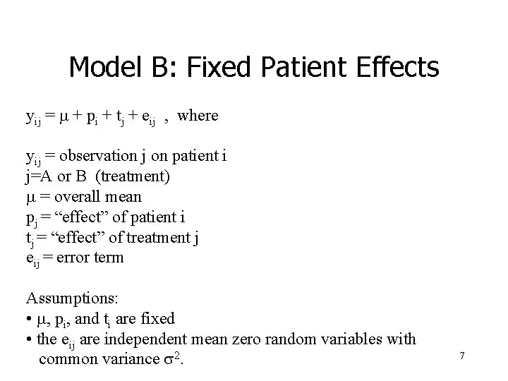
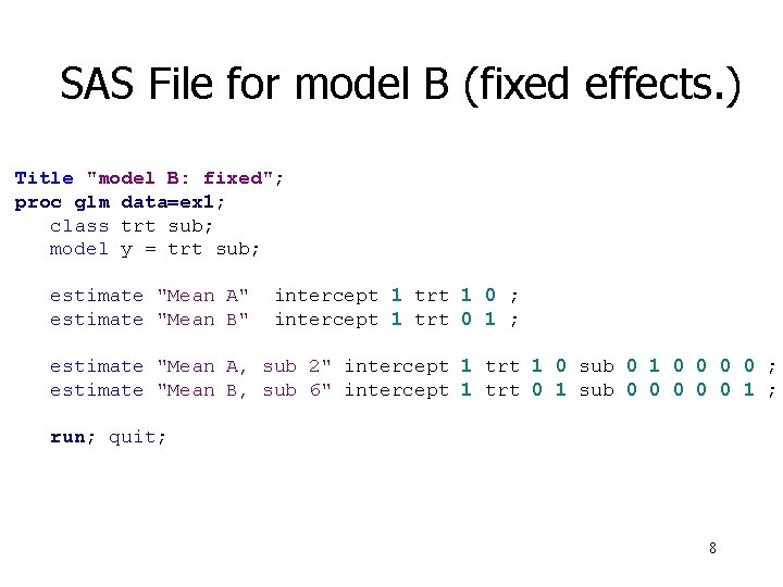
Model B: Fixed Patient Effects yij = m + pi + tj + eij , where yij = observation j on patient i j=A or B (treatment) m = overall mean pj = “effect” of patient i tj = “effect” of treatment j eij = error term Assumptions: • m, pi, and ti are fixed • the eij are independent mean zero random variables with common variance s 2. 7

SAS File for model B (fixed effects. ) Title "model B: fixed"; proc glm data=ex 1; class trt sub; model y = trt sub; estimate "Mean A" estimate "Mean B" intercept 1 trt 1 0 ; intercept 1 trt 0 1 ; estimate "Mean A, sub 2" intercept 1 trt 1 0 sub 0 1 0 0 ; estimate "Mean B, sub 6" intercept 1 trt 0 1 sub 0 0 0 1 ; run; quit; 8

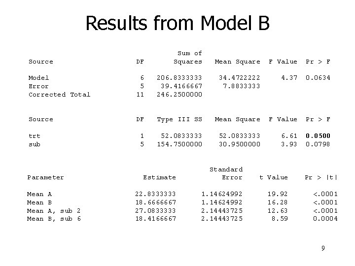
Results from Model B Source DF Sum of Squares Model Error Corrected Total 6 5 11 Source trt sub Parameter Mean A B A, sub 2 B, sub 6 Mean Square F Value Pr > F 206. 8333333 39. 4166667 246. 2500000 34. 4722222 7. 8833333 4. 37 0. 0634 DF Type III SS Mean Square F Value Pr > F 1 5 52. 0833333 154. 7500000 52. 0833333 30. 9500000 6. 61 3. 93 0. 0500 0. 0798 Estimate Standard Error t Value Pr > |t| 22. 8333333 18. 6666667 27. 0833333 18. 4166667 1. 14624992 2. 14443725 19. 92 16. 28 12. 63 8. 59 <. 0001 0. 0004 9

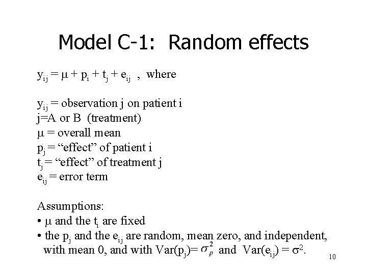
Model C-1: Random effects yij = m + pi + tj + eij , where yij = observation j on patient i j=A or B (treatment) m = overall mean pj = “effect” of patient i tj = “effect” of treatment j eij = error term Assumptions: • m and the ti are fixed • the pj and the eij are random, mean zero, and independent, with mean 0, and with Var(pj)= and Var(eij) = s 2. 10

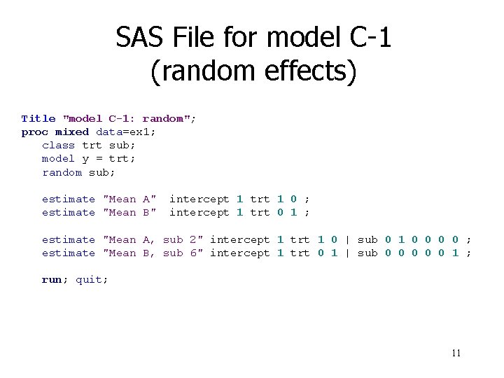
SAS File for model C-1 (random effects) Title "model C-1: random"; proc mixed data=ex 1; class trt sub; model y = trt; random sub; estimate "Mean A" estimate "Mean B" intercept 1 trt 1 0 ; intercept 1 trt 0 1 ; estimate "Mean A, sub 2" intercept 1 trt 1 0 | sub 0 1 0 0 ; estimate "Mean B, sub 6" intercept 1 trt 0 1 | sub 0 0 0 1 ; run; quit; 11

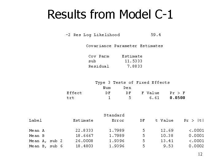
Results from Model C-1 -2 Res Log Likelihood 59. 4 Covariance Parameter Estimates Cov Parm sub Residual Effect trt Label Mean A B A, sub 2 B, sub 6 Estimate 11. 5333 7. 8833 Type 3 Tests of Fixed Effects Num Den DF DF F Value Pr > F 1 5 6. 61 0. 0500 Estimate Standard Error DF t Value Pr > |t| 22. 8333 18. 6667 26. 0008 18. 4803 1. 7989 1. 9396 5 5 12. 69 10. 38 13. 41 9. 53 <. 0001 0. 0001 <. 0001 0. 0002 12

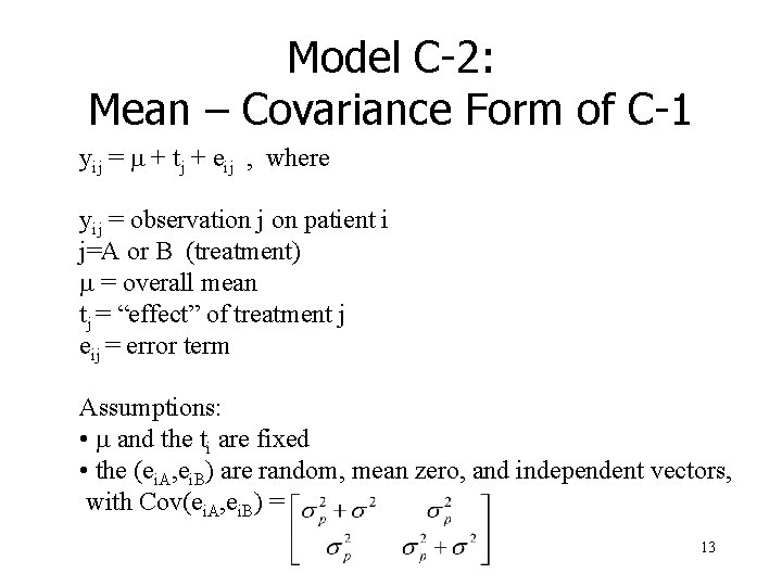
Model C-2: Mean – Covariance Form of C-1 yij = m + tj + eij , where yij = observation j on patient i j=A or B (treatment) m = overall mean tj = “effect” of treatment j eij = error term Assumptions: • m and the ti are fixed • the (ei. A, ei. B) are random, mean zero, and independent vectors, with Cov(ei. A, ei. B) = 13

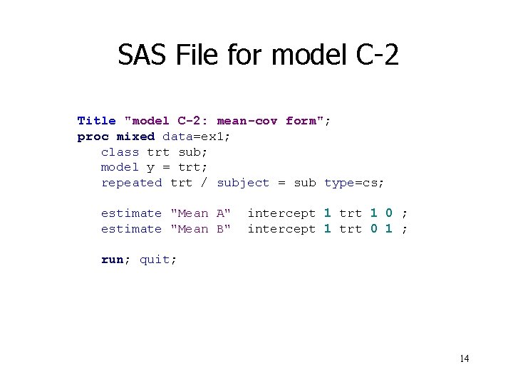
SAS File for model C-2 Title "model C-2: mean-cov form"; proc mixed data=ex 1; class trt sub; model y = trt; repeated trt / subject = sub type=cs; estimate "Mean A" estimate "Mean B" intercept 1 trt 1 0 ; intercept 1 trt 0 1 ; run; quit; 14

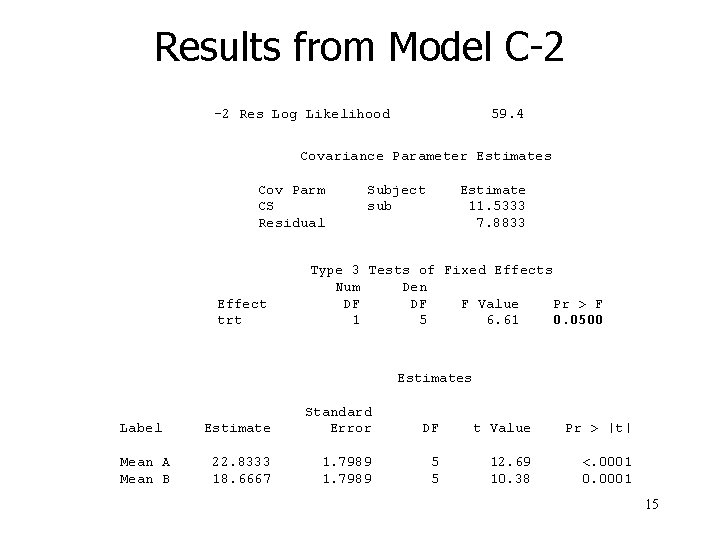
Results from Model C-2 -2 Res Log Likelihood 59. 4 Covariance Parameter Estimates Cov Parm CS Residual Effect trt Subject sub Estimate 11. 5333 7. 8833 Type 3 Tests of Fixed Effects Num Den DF DF F Value Pr > F 1 5 6. 61 0. 0500 Estimates Label Mean A Mean B Estimate Standard Error DF t Value Pr > |t| 22. 8333 18. 6667 1. 7989 5 5 12. 69 10. 38 <. 0001 0. 0001 15

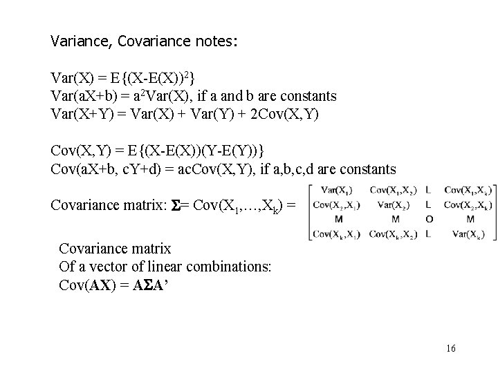
Variance, Covariance notes: Var(X) = E{(X-E(X))2} Var(a. X+b) = a 2 Var(X), if a and b are constants Var(X+Y) = Var(X) + Var(Y) + 2 Cov(X, Y) = E{(X-E(X))(Y-E(Y))} Cov(a. X+b, c. Y+d) = ac. Cov(X, Y), if a, b, c, d are constants Covariance matrix: S= Cov(X 1, …, Xk) = Covariance matrix Of a vector of linear combinations: Cov(AX) = ASA’ 16

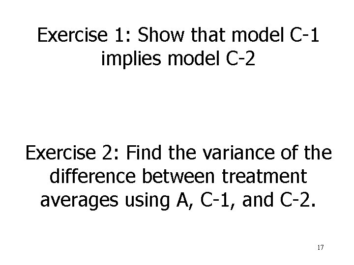
Exercise 1: Show that model C-1 implies model C-2 Exercise 2: Find the variance of the difference between treatment averages using A, C-1, and C-2. 17

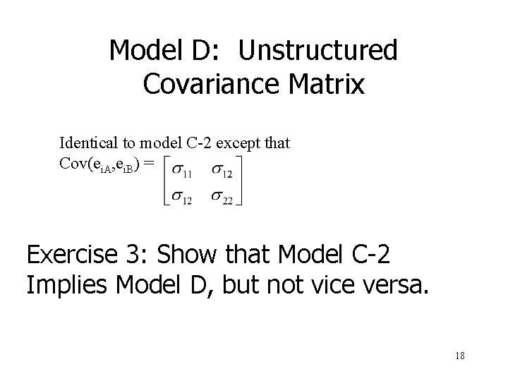
Model D: Unstructured Covariance Matrix Identical to model C-2 except that Cov(ei. A, ei. B) = Exercise 3: Show that Model C-2 Implies Model D, but not vice versa. 18

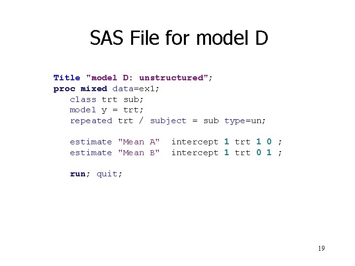
SAS File for model D Title "model D: unstructured"; proc mixed data=ex 1; class trt sub; model y = trt; repeated trt / subject = sub type=un; estimate "Mean A" estimate "Mean B" intercept 1 trt 1 0 ; intercept 1 trt 0 1 ; run; quit; 19

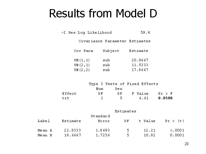
Results from Model D -2 Res Log Likelihood 59. 4 Covariance Parameter Estimates Cov Parm Subject UN(1, 1) UN(2, 2) sub sub Effect trt Estimate 20. 9667 11. 5333 17. 8667 Type 3 Tests of Fixed Effects Num Den DF DF F Value Pr > F 1 5 6. 61 0. 0500 Estimates Label Mean A Mean B Estimate Standard Error DF t Value Pr > |t| 22. 8333 18. 6667 1. 8693 1. 7256 5 5 12. 21 10. 82 <. 0001 0. 0001 20

More exercises Exercise 4: Show to get the standard error for the mean of treatment A in the unstructured model Exercise 5: Find the standard error for the difference between sample means using the unstructured model. 21

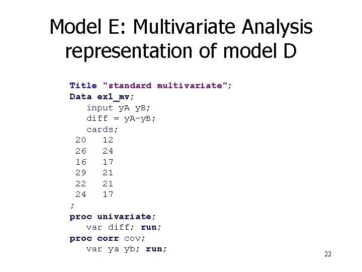
Model E: Multivariate Analysis representation of model D Title "standard multivariate"; Data ex 1_mv; input y. A y. B; diff = y. A-y. B; cards; 20 12 26 24 16 17 29 21 22 21 24 17 ; proc univariate; var diff; run; proc corr cov; var ya yb; run; 22

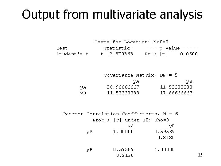
Output from multivariate analysis Test Student's t Tests for Location: Mu 0=0 -Statistic-----p Value-----t 2. 570363 Pr > |t| 0. 0500 Covariance Matrix, DF = 5 y. A y. B 20. 96666667 11. 53333333 17. 86666667 y. A y. B Pearson Correlation Coefficients, N = 6 Prob > |r| under H 0: Rho=0 y. A y. B y. A 1. 00000 0. 59589 0. 2120 y. B 0. 59589 0. 2120 1. 00000 23

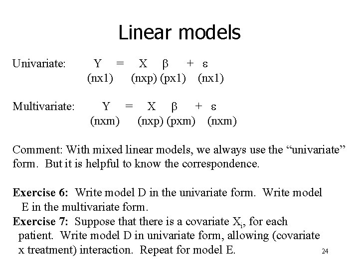
Linear models Univariate: Y = X b + e (nx 1) (nxp) (px 1) (nx 1) Multivariate: Y = X b + e (nxm) (nxp) (pxm) (nxm) Comment: With mixed linear models, we always use the “univariate” form. But it is helpful to know the correspondence. Exercise 6: Write model D in the univariate form. Write model E in the multivariate form. Exercise 7: Suppose that there is a covariate Xi, for each patient. Write model D in univariate form, allowing (covariate 24 x treatment) interaction. Repeat for model E.

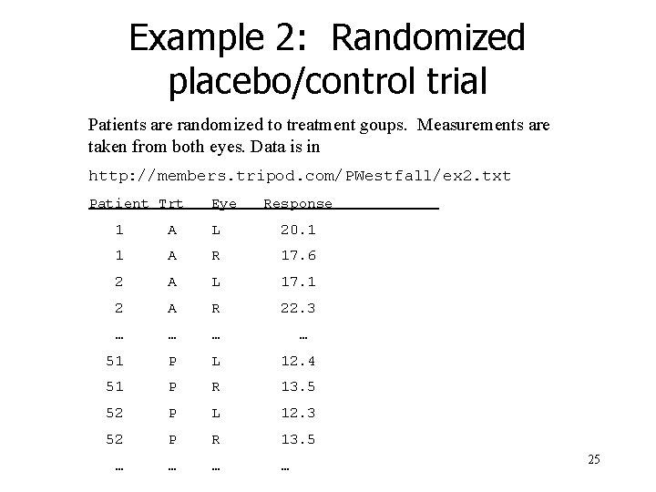
Example 2: Randomized placebo/control trial Patients are randomized to treatment goups. Measurements are taken from both eyes. Data is in http: //members. tripod. com/PWestfall/ex 2. txt Patient Trt Eye Response 1 A L 20. 1 1 A R 17. 6 2 A L 17. 1 2 A R 22. 3 … … 51 P L 12. 4 51 P R 13. 5 52 P L 12. 3 52 P R 13. 5 … … 25

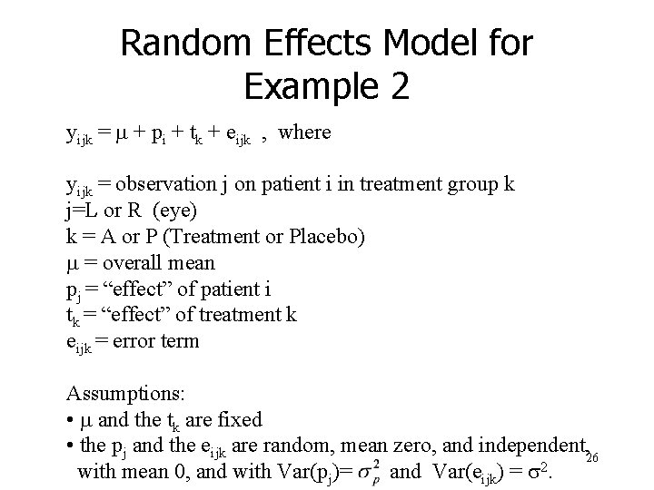
Random Effects Model for Example 2 yijk = m + pi + tk + eijk , where yijk = observation j on patient i in treatment group k j=L or R (eye) k = A or P (Treatment or Placebo) m = overall mean pj = “effect” of patient i tk = “effect” of treatment k eijk = error term Assumptions: • m and the tk are fixed • the pj and the eijk are random, mean zero, and independent, 26 with mean 0, and with Var(pj)= and Var(eijk) = s 2.

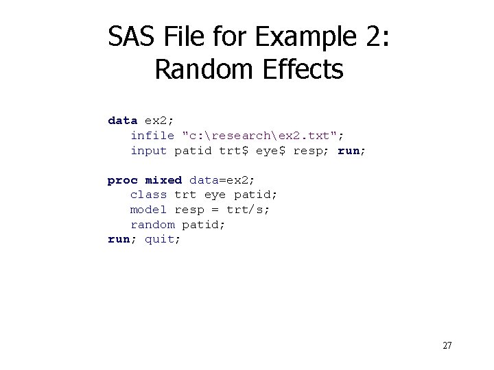
SAS File for Example 2: Random Effects data ex 2; infile "c: researchex 2. txt"; input patid trt$ eye$ resp; run; proc mixed data=ex 2; class trt eye patid; model resp = trt/s; random patid; run; quit; 27

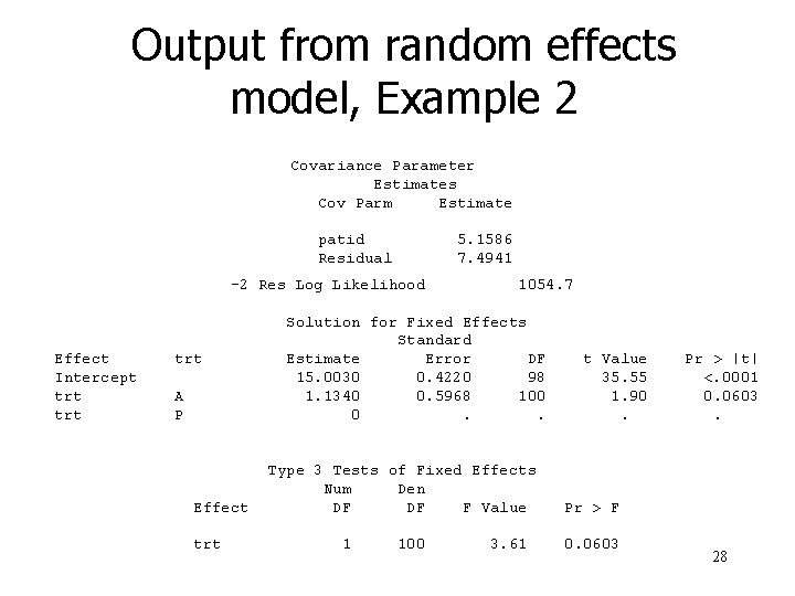
Output from random effects model, Example 2 Covariance Parameter Estimates Cov Parm Estimate patid Residual 5. 1586 7. 4941 -2 Res Log Likelihood Effect Intercept trt trt A P Effect trt 1054. 7 Solution for Fixed Effects Standard Estimate Error DF 15. 0030 0. 4220 98 1. 1340 0. 5968 100 0. . Type 3 Tests of Fixed Effects Num Den DF DF F Value 1 100 3. 61 t Value 35. 55 1. 90. Pr > |t| <. 0001 0. 0603. Pr > F 0. 0603 28

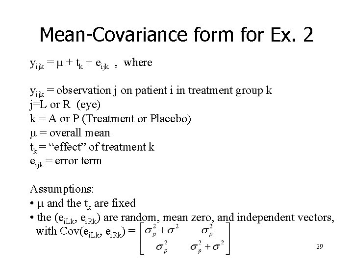
Mean-Covariance form for Ex. 2 yijk = m + tk + eijk , where yijk = observation j on patient i in treatment group k j=L or R (eye) k = A or P (Treatment or Placebo) m = overall mean tk = “effect” of treatment k eijk = error term Assumptions: • m and the tk are fixed • the (ei. Lk, ei. Rk) are random, mean zero, and independent vectors, with Cov(ei. Lk, ei. Rk) = 29

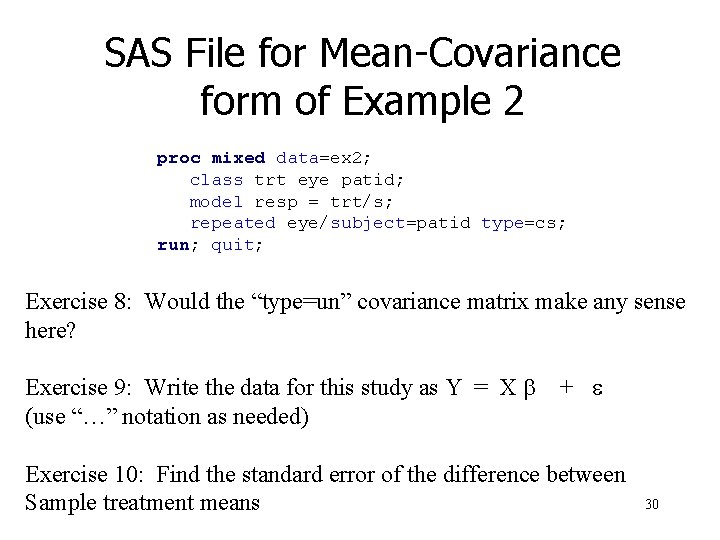
SAS File for Mean-Covariance form of Example 2 proc mixed data=ex 2; class trt eye patid; model resp = trt/s; repeated eye/subject=patid type=cs; run; quit; Exercise 8: Would the “type=un” covariance matrix make any sense here? Exercise 9: Write the data for this study as Y = X b + e (use “…” notation as needed) Exercise 10: Find the standard error of the difference between Sample treatment means 30

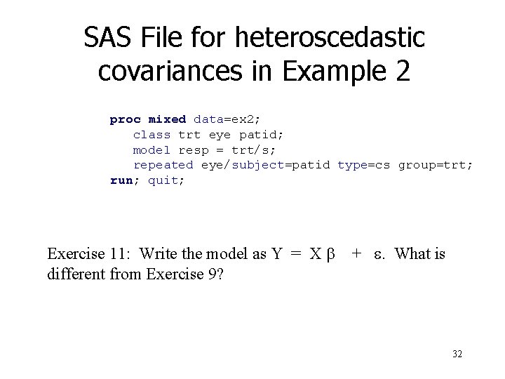
Fitting heteroscedastic covariance matrices Model: Same as the mean-covariance form for ex. 2, but with Cov(ei. LA, ei. RA) = And Cov(ei. LP, ei. RP) = 31

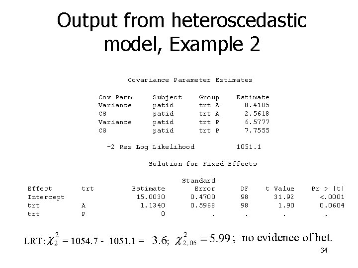
SAS File for heteroscedastic covariances in Example 2 proc mixed data=ex 2; class trt eye patid; model resp = trt/s; repeated eye/subject=patid type=cs group=trt; run; quit; Exercise 11: Write the model as Y = X b + e. What is different from Exercise 9? 32

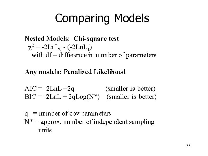
Comparing Models Nested Models: Chi-square test c 2 = -2 Ln. L 0 - (-2 Ln. L 1) with df = difference in number of parameters Any models: Penalized Likelihood AIC = -2 Ln. L +2 q (smaller-is-better) BIC = -2 Ln. L + 2 q. Log(N*) (smaller-is-better) q = number of cov parameters N* = approx. number of independent sampling units 33

Output from heteroscedastic model, Example 2 Covariance Parameter Estimates Cov Parm Variance CS Subject patid Group trt A trt P -2 Res Log Likelihood Estimate 8. 4105 2. 5618 6. 5777 7. 7555 1051. 1 Solution for Fixed Effects Effect Intercept trt trt A P Estimate 15. 0030 1. 1340 0 LRT: = 1054. 7 - 1051. 1 = 3. 6; Standard Error 0. 4700 0. 5968. DF 98 98. t Value 31. 92 1. 90. Pr > |t| <. 0001 0. 0604. ; no evidence of het. 34

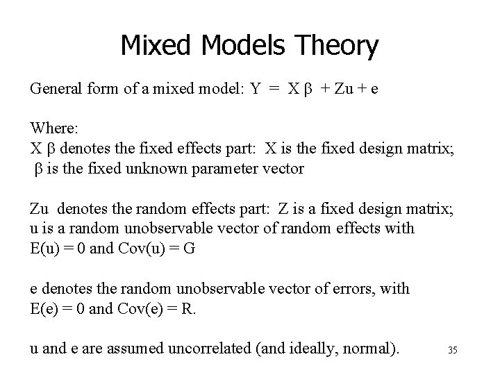
Mixed Models Theory General form of a mixed model: Y = X b + Zu + e Where: X b denotes the fixed effects part: X is the fixed design matrix; b is the fixed unknown parameter vector Zu denotes the random effects part: Z is a fixed design matrix; u is a random unobservable vector of random effects with E(u) = 0 and Cov(u) = G e denotes the random unobservable vector of errors, with E(e) = 0 and Cov(e) = R. u and e are assumed uncorrelated (and ideally, normal). 35

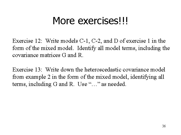
More exercises!!! Exercise 12: Write models C-1, C-2, and D of exercise 1 in the form of the mixed model. Identify all model terms, including the covariance matrices G and R. Exercise 13: Write down the heteroscedastic covariance model from example 2 in the form of the mixed model, identifying all terms, including G and R. Use “…” as needed. 36

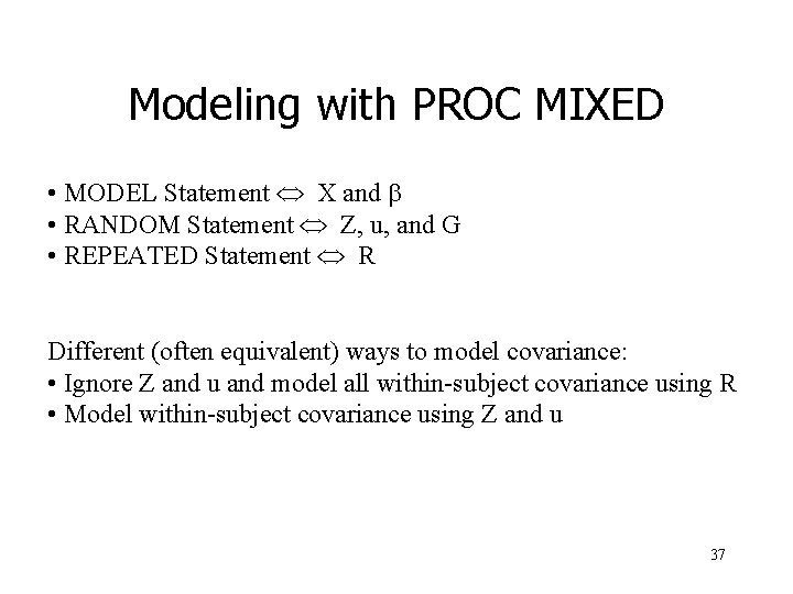
Modeling with PROC MIXED • MODEL Statement Û X and b • RANDOM Statement Û Z, u, and G • REPEATED Statement Û R Different (often equivalent) ways to model covariance: • Ignore Z and u and model all within-subject covariance using R • Model within-subject covariance using Z and u 37

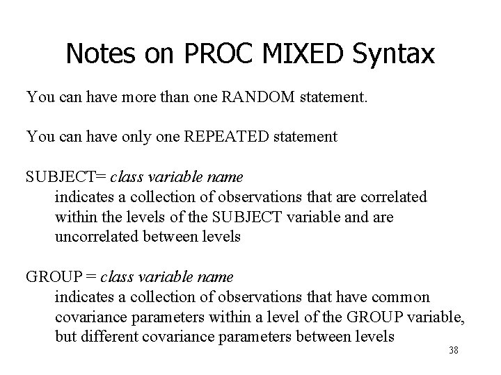
Notes on PROC MIXED Syntax You can have more than one RANDOM statement. You can have only one REPEATED statement SUBJECT= class variable name indicates a collection of observations that are correlated within the levels of the SUBJECT variable and are uncorrelated between levels GROUP = class variable name indicates a collection of observations that have common covariance parameters within a level of the GROUP variable, but different covariance parameters between levels 38

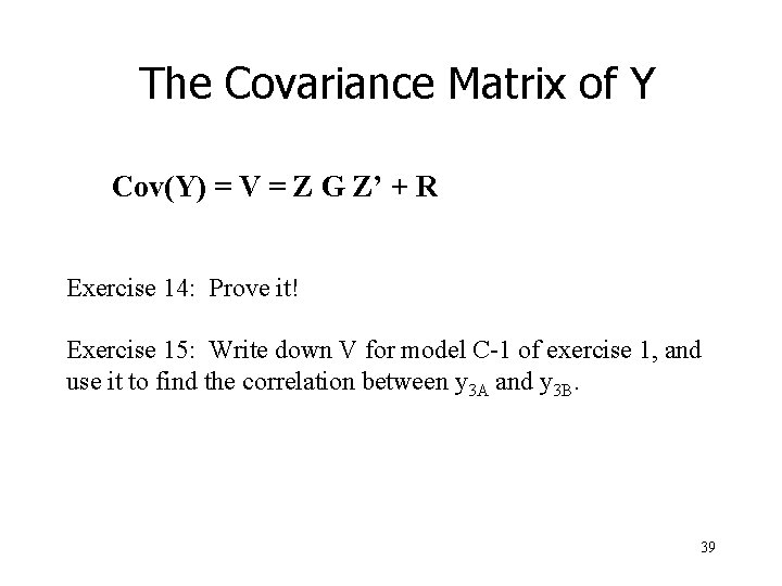
The Covariance Matrix of Y Cov(Y) = V = Z G Z’ + R Exercise 14: Prove it! Exercise 15: Write down V for model C-1 of exercise 1, and use it to find the correlation between y 3 A and y 3 B. 39

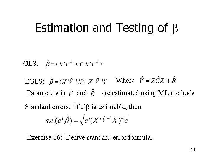
Estimation and Testing of b GLS: Where EGLS: Parameters in and are estimated using ML methods Standard errors: if c’b is estimable, then Exercise 16: Derive standard error formula. 40

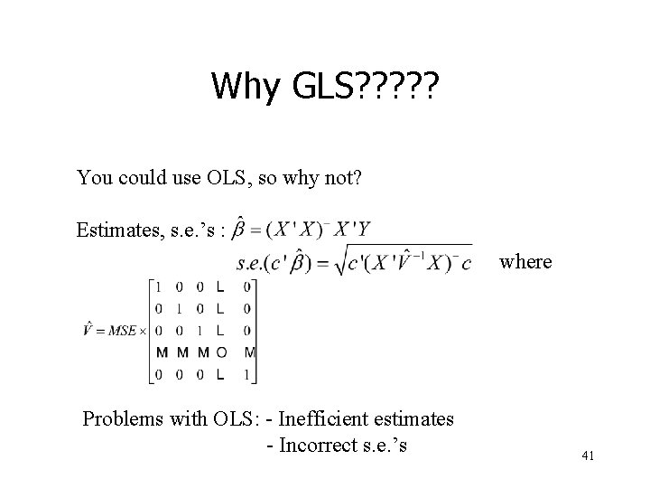
Why GLS? ? ? You could use OLS, so why not? Estimates, s. e. ’s : where Problems with OLS: - Inefficient estimates - Incorrect s. e. ’s 41

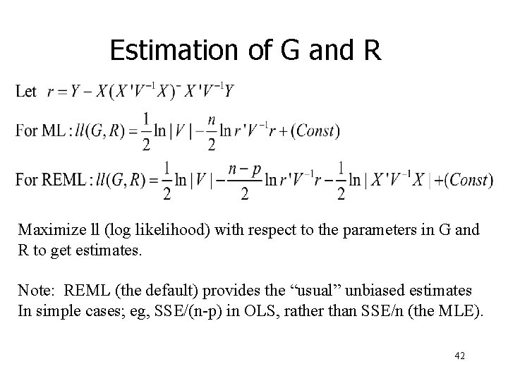
Estimation of G and R Maximize ll (log likelihood) with respect to the parameters in G and R to get estimates. Note: REML (the default) provides the “usual” unbiased estimates In simple cases; eg, SSE/(n-p) in OLS, rather than SSE/n (the MLE). 42

Modeling a Multi-Center Clinical Trial Data: Baseline Diastolic Blood Pressure (dbp) on each patient Nine-week dbp measure (LOCF) Treatments A, B, and C Data come from 35 centers (1 – 40 patients per center) 43

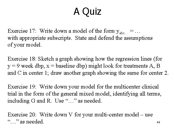
A Quiz Exercise 17: Write down a model of the form yabc… = … with appropriate subscripts. State and defend the assumptions of your model. Exercise 18: Sketch a graph showing how the regression lines (for y = 9 week dbp, x = baseline dbp) might look for treatments A, B and C in center 1; draw another graph showing the same for center 2. Exercise 19: Write down your model for the multicenter clinical trial in the form of the general mixed model, identifying all terms, including G and R. Use “…” as needed. Exercise 20: Write down V for your multi-center model – use “…” as needed. 44

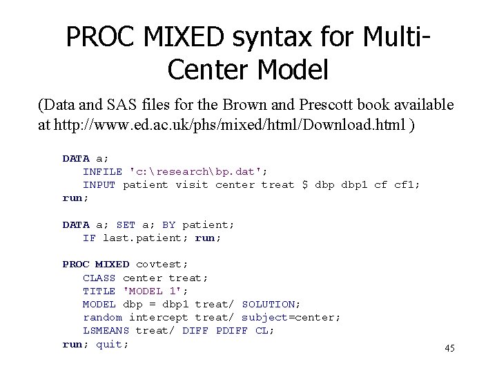
PROC MIXED syntax for Multi. Center Model (Data and SAS files for the Brown and Prescott book available at http: //www. ed. ac. uk/phs/mixed/html/Download. html ) DATA a; INFILE 'c: researchbp. dat'; INPUT patient visit center treat $ dbp 1 cf cf 1; run; DATA a; SET a; BY patient; IF last. patient; run; PROC MIXED covtest; CLASS center treat; TITLE 'MODEL 1'; MODEL dbp = dbp 1 treat/ SOLUTION; random intercept treat/ subject=center; LSMEANS treat/ DIFF PDIFF CL; run; quit; 45

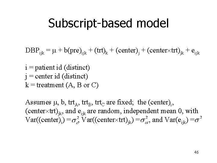
Subscript-based model DBPijk = m + b(pre)ijk + (trt)k + (center)j + (center´trt)jk + eijk i = patient id (distinct) j = center id (distinct) k = treatment (A, B or C) Assumes m, b, trt. A, trt. B, trt. C are fixed; the (center)i, (center´trt)jk, and eijk are random, independent mean 0, with Var((center)i) = , Var((center´trt)jk) = , and Var(eijk) = 46

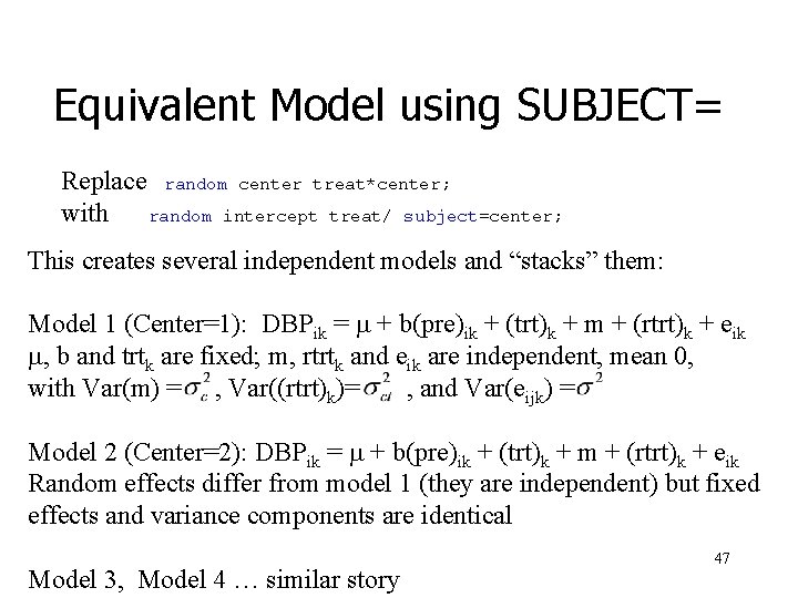
Equivalent Model using SUBJECT= Replace random center treat*center; with random intercept treat/ subject=center; This creates several independent models and “stacks” them: Model 1 (Center=1): DBPik = m + b(pre)ik + (trt)k + m + (rtrt)k + eik m, b and trtk are fixed; m, rtrtk and eik are independent, mean 0, with Var(m) = , Var((rtrt)k)= , and Var(eijk) = Model 2 (Center=2): DBPik = m + b(pre)ik + (trt)k + m + (rtrt)k + eik Random effects differ from model 1 (they are independent) but fixed effects and variance components are identical Model 3, Model 4 … similar story 47

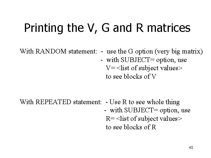
Printing the V, G and R matrices With RANDOM statement: - use the G option (very big matrix) - with SUBJECT= option, use V= <list of subject values> to see blocks of V With REPEATED statement: - Use R to see whole thing - with SUBJECT= option, use R= <list of subject values> to see blocks of R 48

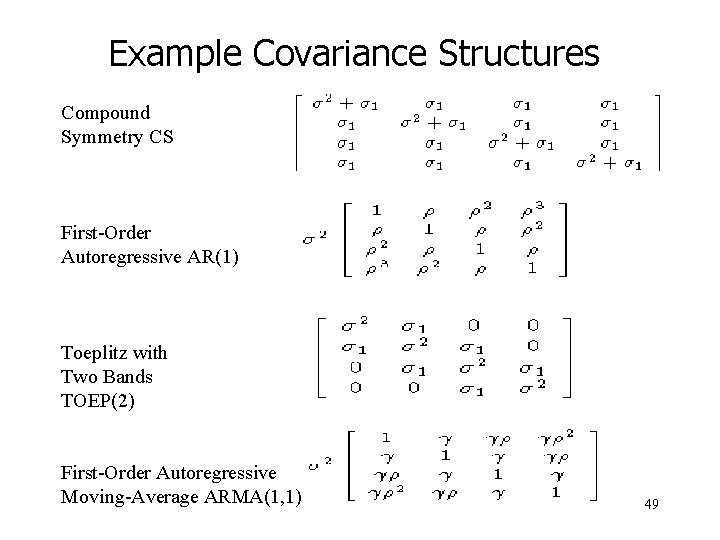
Example Covariance Structures Compound Symmetry CS First-Order Autoregressive AR(1) Toeplitz with Two Bands TOEP(2) First-Order Autoregressive Moving-Average ARMA(1, 1) 49

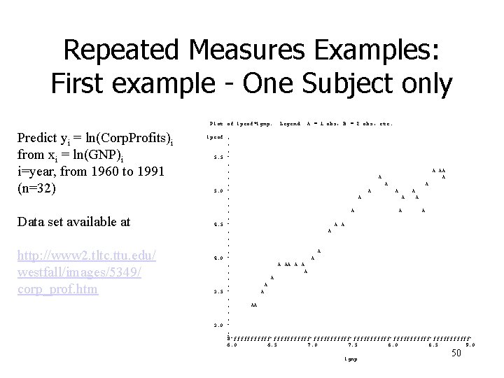
Repeated Measures Examples: First example - One Subject only Plot of lprof*lgnp. Predict yi = ln(Corp. Profits)i from xi = ln(GNP)i i=year, from 1960 to 1991 (n=32) Data set available at http: //www 2. tltc. ttu. edu/ westfall/images/5349/ corp_prof. htm Legend: A = 1 obs, B = 2 obs, etc. lprof ‚ ‚ ‚ 5. 5 ˆ ‚ ‚ A AA ‚ A A 5. 0 ˆ A A A ‚ ‚ A A A ‚ 4. 5 ˆ A A ‚ ‚ ‚ A 4. 0 ˆ A ‚ A AA A A ‚ A ‚ A 3. 5 ˆ A ‚ ‚ AA ‚ ‚ 3. 0 ˆ ‚ Šˆƒƒƒƒƒƒƒƒƒƒƒˆƒƒƒƒƒƒƒƒƒƒƒˆƒƒƒƒƒƒƒƒƒƒƒˆ 6. 0 6. 5 7. 0 7. 5 8. 0 8. 5 9. 0 lgnp 50

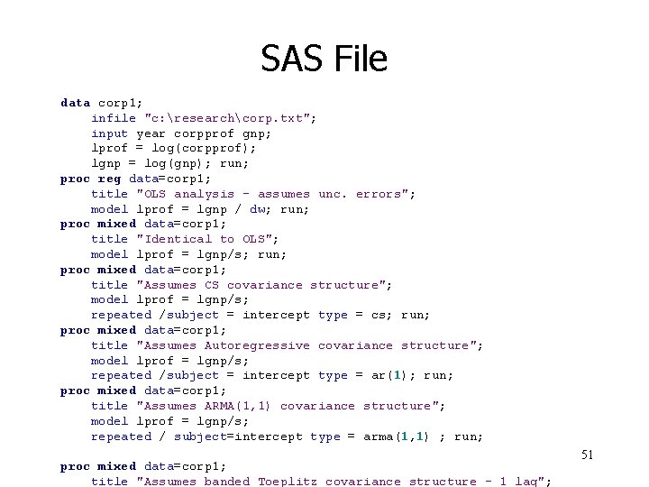
SAS File data corp 1; infile "c: researchcorp. txt"; input year corpprof gnp; lprof = log(corpprof); lgnp = log(gnp); run; proc reg data=corp 1; title "OLS analysis - assumes unc. errors"; model lprof = lgnp / dw; run; proc mixed data=corp 1; title "Identical to OLS"; model lprof = lgnp/s; run; proc mixed data=corp 1; title "Assumes CS covariance structure"; model lprof = lgnp/s; repeated /subject = intercept type = cs; run; proc mixed data=corp 1; title "Assumes Autoregressive covariance structure"; model lprof = lgnp/s; repeated /subject = intercept type = ar(1); run; proc mixed data=corp 1; title "Assumes ARMA(1, 1) covariance structure"; model lprof = lgnp/s; repeated / subject=intercept type = arma(1, 1) ; run; proc mixed data=corp 1; title "Assumes banded Toeplitz covariance structure - 1 lag"; 51

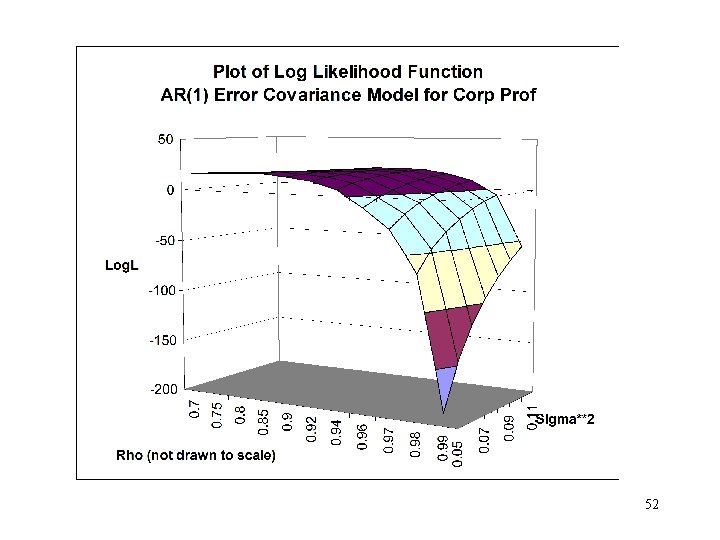
52

Quiz Exercise 21: Write down the AR(1) corp profits model using “subscript” notation. State all model assumptions and defend (or criticize) them. Exercise 22: Identify Y, X, Z, u, b, G and R for the AR(1) corp profits model. Use “…” as needed. Exercise 23: Repeat exercise 20 and 21 for the CS model. Exercise 24: Write the CS model as a “random effects” model. Use this model to show why there is a problem with using the CS model for these data. 53

Repeated Measures: Multiple Subjects Case description: Workers perform various lifting tasks throughout the day. There is an amount of stress associated with each lift. Ergonomists have defined various measurements of stress. In the data set there are two such measures; one is called li 81 (published in 1981) and the other is li 91 (published in 91). The input data has the logs of these stress measures. The funding agency wants to know if the li 81 measure is predictive of the li 91 measure. Our analysis must account for the repeated measures on each subject, which implies that the observations within a person are correlated. http: //www 2. tltc. ttu. edu/westfall/images/5349/li%20 case_description. htm 54

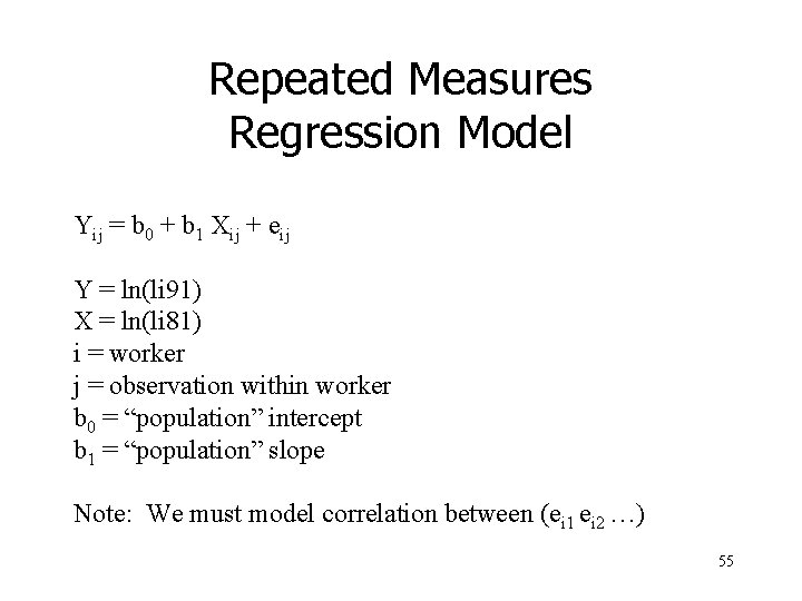
Repeated Measures Regression Model Yij = b 0 + b 1 Xij + eij Y = ln(li 91) X = ln(li 81) i = worker j = observation within worker b 0 = “population” intercept b 1 = “population” slope Note: We must model correlation between (ei 1 ei 2 …) 55

Quiz Exercise 25: Write down the random effects model in “subscript” form that will allow a CS covariance matrix. Write the CLASS, MODEL and RANDOM statements To correspond. Exercise 26: Write down the model in “mean and covariance matrix form” to allow a CS covariance matrix. Write the CLASS, MODEL and REPEATED statements to correspond. 56

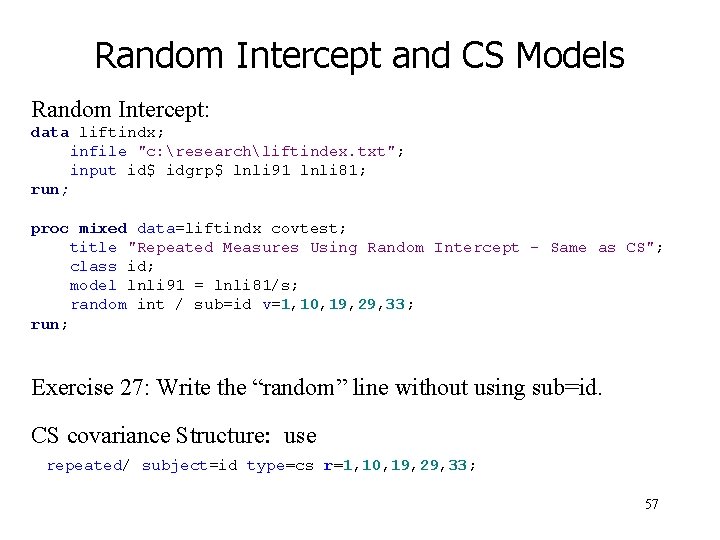
Random Intercept and CS Models Random Intercept: data liftindx; infile "c: researchliftindex. txt"; input id$ idgrp$ lnli 91 lnli 81; run; proc mixed data=liftindx covtest; title "Repeated Measures Using Random Intercept - Same as CS"; class id; model lnli 91 = lnli 81/s; random int / sub=id v=1, 10, 19, 29, 33; run; Exercise 27: Write the “random” line without using sub=id. CS covariance Structure: use repeated/ subject=id type=cs r=1, 10, 19, 29, 33; 57

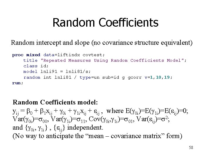
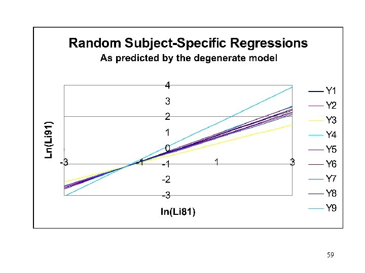
Random Coefficients Random intercept and slope (no covariance structure equivalent) proc mixed data=liftindx covtest; title "Repeated Measures Using Random Coefficients Model"; class id; model lnli 91 = lnli 81/s; random int lnli 81 / type=un sub=id g gcorr v=1, 10, 19; run; Random Coefficients model: yij = b 0 + b 1 xij + g 0 i + g 1 ixij + eij , where E(g 0 i)=E(g 1 i)=E(eij)=0; Var(g 0 i)=s 00, Var(g 1 i)=s 11, Cov(g 0 i, g 1 i)=s 01, Var(eij)=s 2; and {g 0 i, g 1 i} , {eij} independent. (No way to anticipate the “mean – covariance matrix” form) 58

59

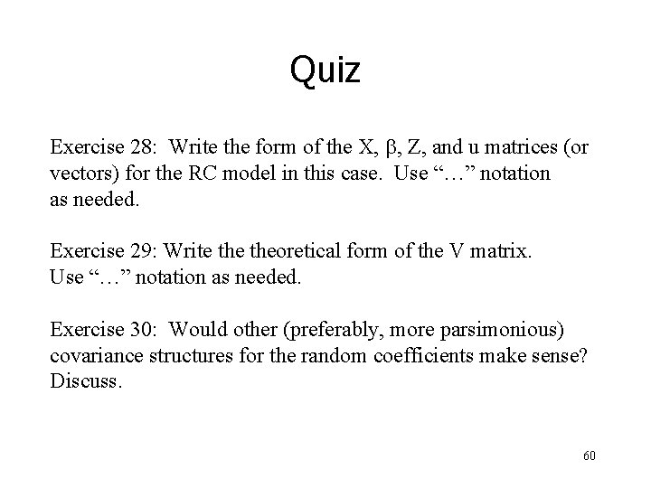
Quiz Exercise 28: Write the form of the X, b, Z, and u matrices (or vectors) for the RC model in this case. Use “…” notation as needed. Exercise 29: Write theoretical form of the V matrix. Use “…” notation as needed. Exercise 30: Would other (preferably, more parsimonious) covariance structures for the random coefficients make sense? Discuss. 60

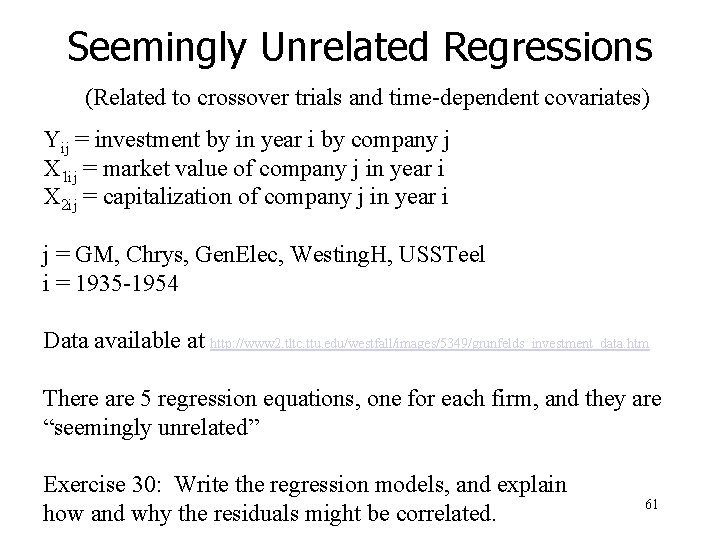
Seemingly Unrelated Regressions (Related to crossover trials and time-dependent covariates) Yij = investment by in year i by company j X 1 ij = market value of company j in year i X 2 ij = capitalization of company j in year i j = GM, Chrys, Gen. Elec, Westing. H, USSTeel i = 1935 -1954 Data available at http: //www 2. tltc. ttu. edu/westfall/images/5349/grunfelds_investment_data. htm There are 5 regression equations, one for each firm, and they are “seemingly unrelated” Exercise 30: Write the regression models, and explain how and why the residuals might be correlated. 61

Missing Data In SUR One beauty of the Mixed Model approach is that complete cases are not needed – you can use all of the data that you have. Caveat: Missing cases should be missing AT RANDOM! (the bad news is that this assumption is frequently not satisfied!) Example: Investment data, with data for various companies Missing at particular years. 62

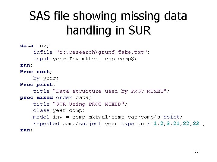
SAS file showing missing data handling in SUR data inv; infile "c: researchgrunf_fake. txt"; input year Inv mktval cap comp$; run; Proc sort; by year; Proc print; title "Data structure used by PROC MIXED"; proc mixed order=data; title "SUR Using PROC MIXED"; class year comp; model inv = comp mktval*comp cap*comp/s noint; repeated comp/subject=year type=un r=1, 2, 3, 21, 22, 23 ; run; 63

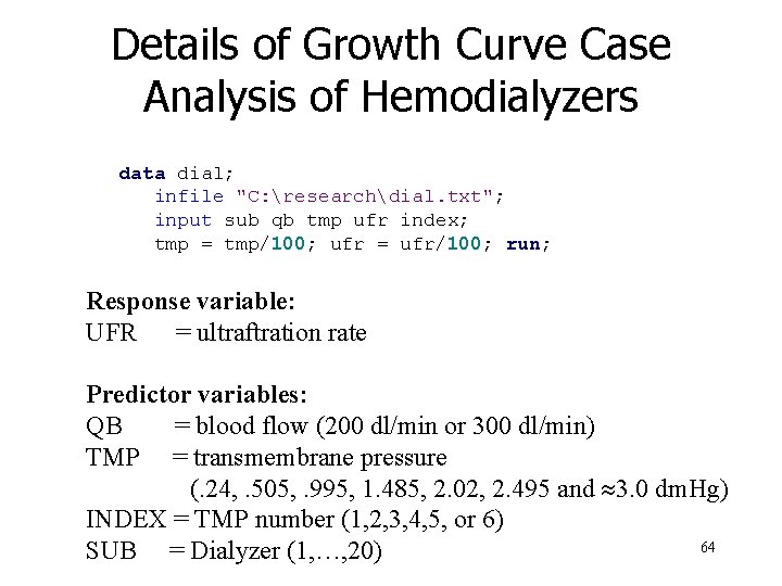
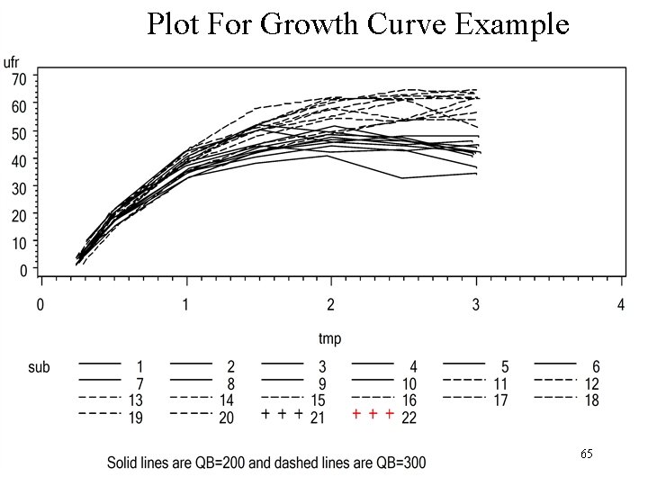
Details of Growth Curve Case Analysis of Hemodialyzers data dial; infile "C: researchdial. txt"; input sub qb tmp ufr index; tmp = tmp/100; ufr = ufr/100; run; Response variable: UFR = ultraftration rate Predictor variables: QB = blood flow (200 dl/min or 300 dl/min) TMP = transmembrane pressure (. 24, . 505, . 995, 1. 485, 2. 02, 2. 495 and » 3. 0 dm. Hg) INDEX = TMP number (1, 2, 3, 4, 5, or 6) 64 SUB = Dialyzer (1, …, 20)

Plot For Growth Curve Example 65

Quiz!!!! Exercise 31: Write a mixed model to predict UFR. What assumptions are you making? Do those assumptions seem reasonable? Exercise 32: Write the SAS PROC MIXED code needed to fit your growth curve model. 66

BLUPs Example: Consider estimating the means of treatment A in the blood pressure trial for different centers. Objective: Rank the centers according to average dbp in their patient populations. Problem: The simple averages may be inappropriate when the number of patients per center varies. Solution: Rank centers using BLUPs (best linear unbiased predictors), which shrink the estimates toward an overall mean. 67

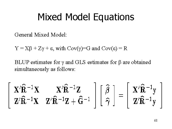
Mixed Model Equations General Mixed Model: Y = Xb + Zg + e, with Cov(g)=G and Cov(e) = R BLUP estimates for g and GLS estimates for b are obtained simultaneously as follows: 68

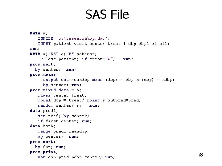
SAS File DATA a; INFILE 'c: researchbp. dat'; INPUT patient visit center treat $ dbp 1 cf cf 1; run; DATA a; SET a; BY patient; IF last. patient; if treat="A"; run; proc sort; by center; run; proc means; output out=meandbp mean (dbp) = dbp n (dbp) = ndbp; by center; run; proc mixed data = a; class center treat; model dbp = treat/ noint s outpred=pred; random center/ s; run; data pred 1; set pred; by center; if first. center; run; data both; merge pred 1 meandbp; by center; run; proc sort; by dbp; run; proc print; var dbp pred ndbp center; run; 69

Final Words • Mixed Model Methodology provides a powerful, flexible tool for estimating effects with repeated measures data • Likelihood-based methodology allows for simple model comparisons • Caveats: The methods are suspect with – Gross nonnormality – Badly misspecified covariance structure (including non-modelled heteroscedasticity) – Data missing not at random – Nonlinearity – Omitted variable bias – Confounding 70