Introduction to MATLAB Farida Mosally Mathematics Department King

Introduction to MATLAB Farida Mosally Mathematics Department King Abdulaziz University 2013

Out Line This introduction will gives • • • Starting a MATLAB Matrices and Arrays Graphics Symbolic Math Toolbox Control Flow and if Statement Functions 3

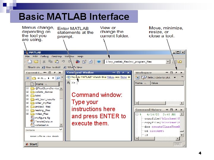
Basic MATLAB Interface Command window: Type your instructions here and press ENTER to execute them. 4

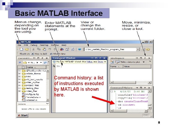
Basic MATLAB Interface Command history: a list of instructions executed by MATLAB is shown here. 5

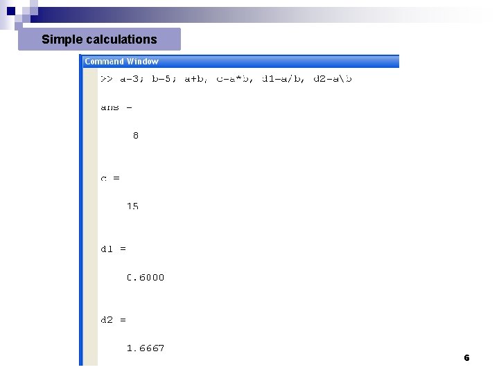
Simple calculations 6

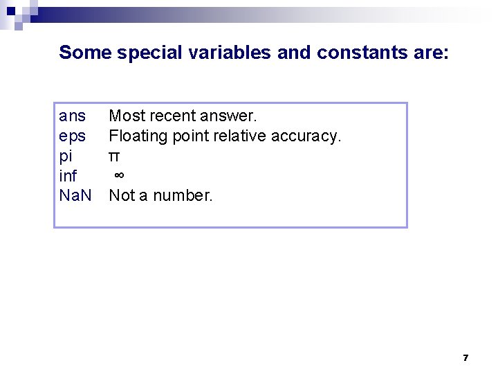
Some special variables and constants are: ans eps pi inf Na. N Most recent answer. Floating point relative accuracy. π ∞ Not a number. 7

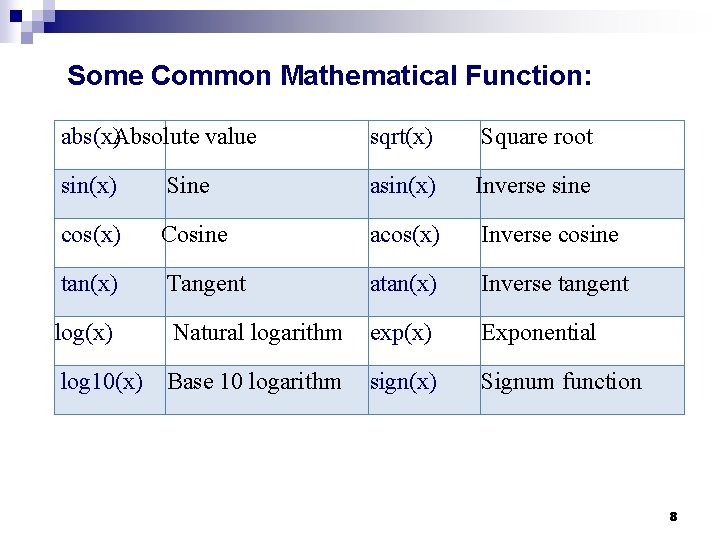
Some Common Mathematical Function: abs(x)Absolute value sqrt(x) Square root sin(x) Sine asin(x) Inverse sine cos(x) Cosine acos(x) Inverse cosine tan(x) Tangent atan(x) Inverse tangent log(x) Natural logarithm exp(x) Exponential log 10(x) Base 10 logarithm sign(x) Signum function 8

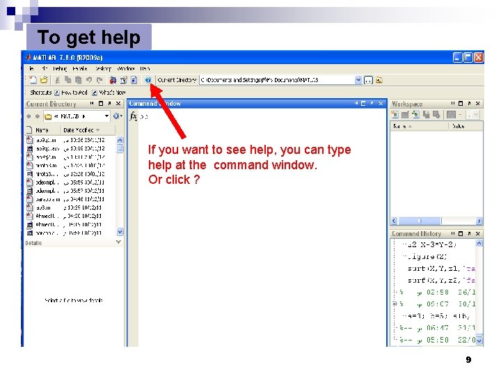
To get help If you want to see help, you can type help at the command window. Or click ? 9

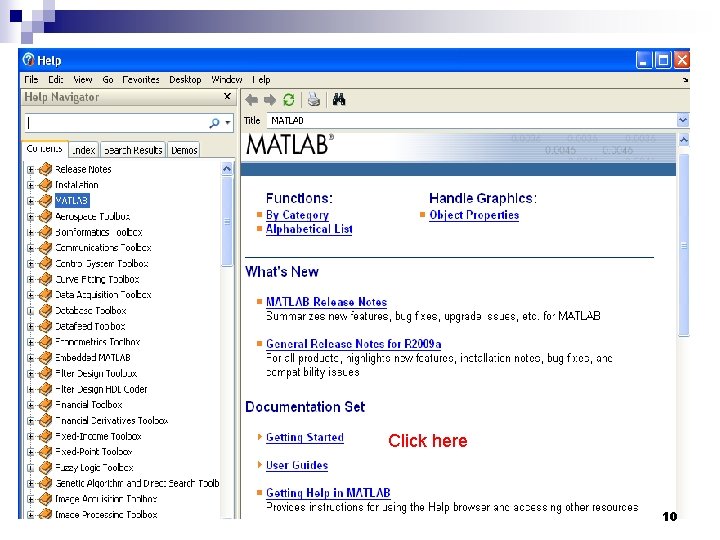
Click here 10

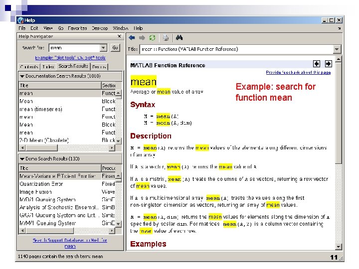
Example: search for function mean 11

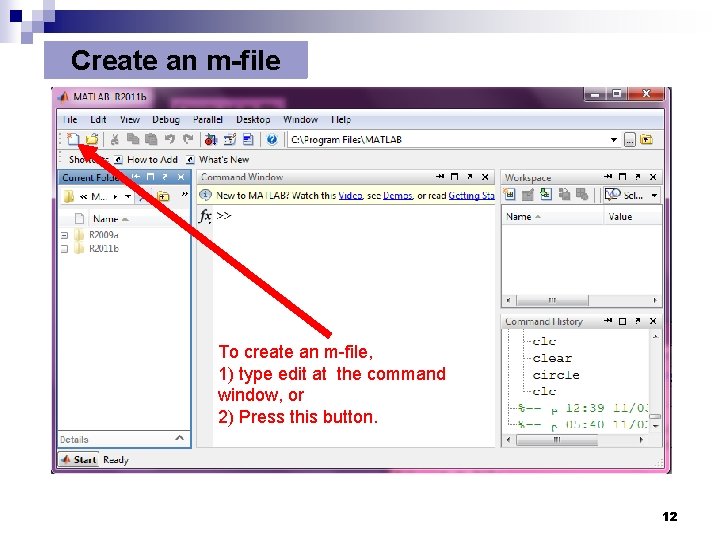
Create an m-file To create an m-file, 1) type edit at the command window, or 2) Press this button. 12

Create an m-file The previous command will display the editor window. The editor creates an m-file that can be used to write your MATLAB programs. 13

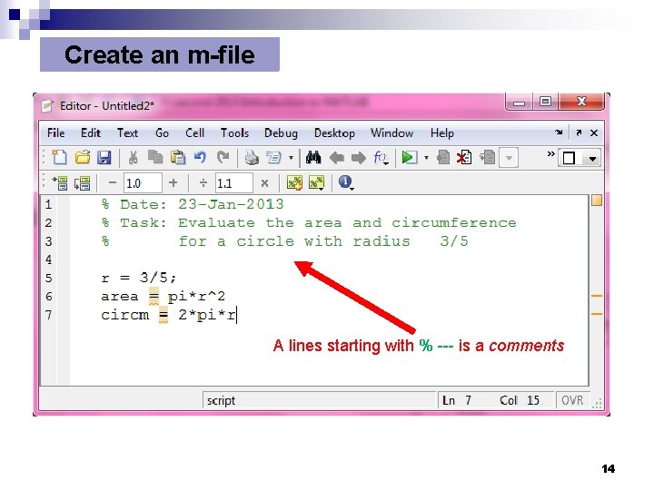
Create an m-file A lines starting with % --- is a comments 14

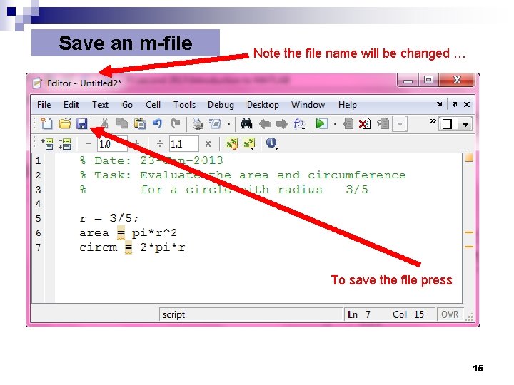
Save an m-file Note the file name will be changed … To save the file press 15

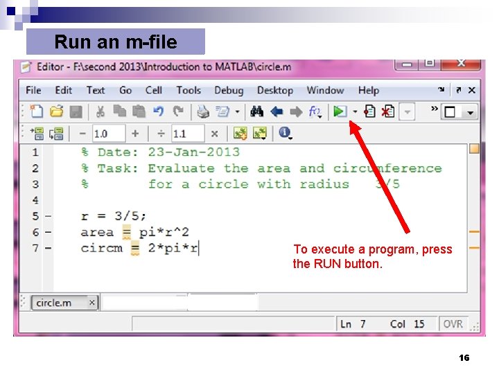
Run an m-file To execute a program, press the RUN button. 16

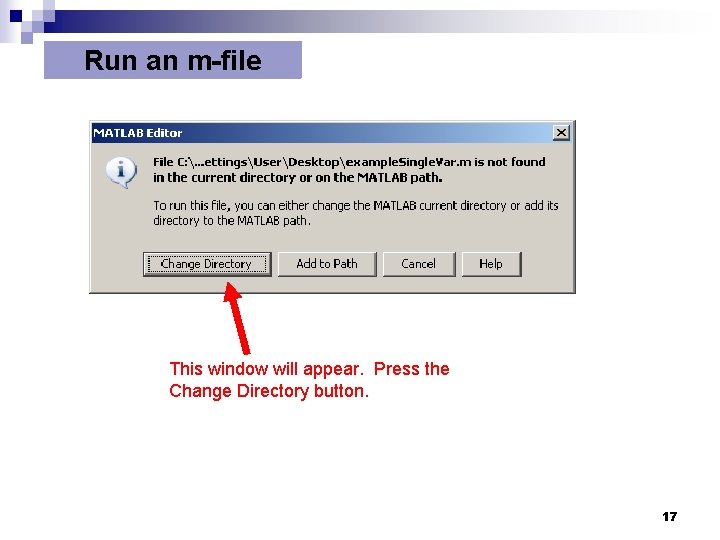
Run an m-file This window will appear. Press the Change Directory button. 17

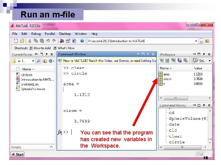
Run an m-file You can see that the program has created new variables in the Workspace. 18

Matrices and Arrays

Simple Arrays >> V = [1 3, sqrt(5)] V= 1. 0000 3. 0000 2. 2361 >> A = [1 2 3; 4 5 6; 7 8 0] A= 1 2 3 4 5 6 7 8 0 20

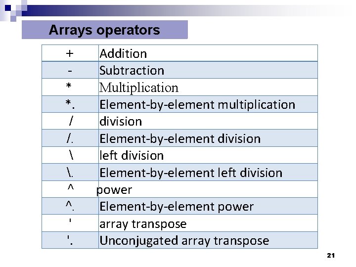
Arrays operators + * *. / /. . ^ ^. ' '. Addition Subtraction Multiplication Element-by-element multiplication division Element-by-element division left division Element-by-element left division power Element-by-element power array transpose Unconjugated array transpose 21

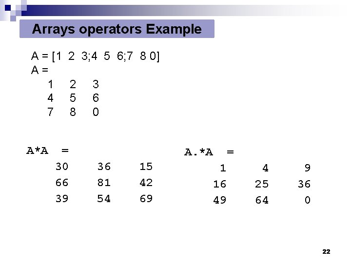
Arrays operators Example A = [1 A= 1 4 7 A*A 2 3; 4 5 6; 7 8 0] = 30 66 39 2 5 8 3 6 0 A. *A 36 81 54 15 42 69 = 1 16 49 4 25 64 9 36 0 22

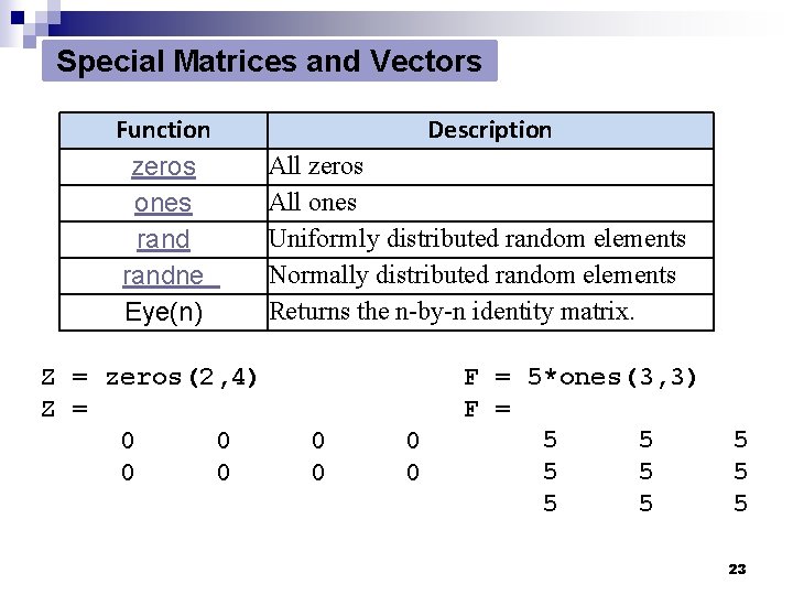
Special Matrices and Vectors Function zeros ones randne Eye(n) Z = zeros(2, 4) Z = 0 0 Description All zeros All ones Uniformly distributed random elements Normally distributed random elements Returns the n-by-n identity matrix. 0 0 F = 5*ones(3, 3) F = 5 5 5 5 5 23

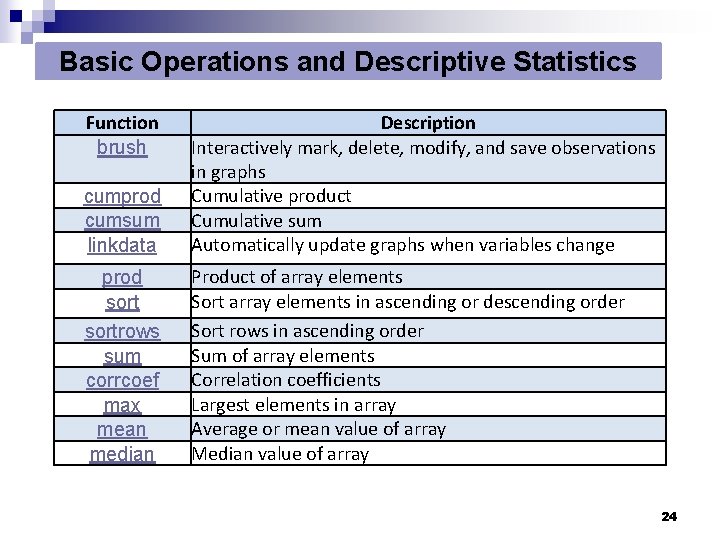
Basic Operations and Descriptive Statistics Function brush cumprod cumsum linkdata Description Interactively mark, delete, modify, and save observations in graphs Cumulative product Cumulative sum Automatically update graphs when variables change prod sortrows sum corrcoef max mean median Product of array elements Sort array elements in ascending or descending order Sort rows in ascending order Sum of array elements Correlation coefficients Largest elements in array Average or mean value of array Median value of array 24

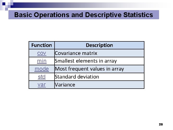
Basic Operations and Descriptive Statistics Function cov min mode std var Description Covariance matrix Smallest elements in array Most frequent values in array Standard deviation Variance 25

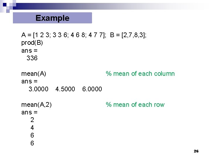
Example A = [1 2 3; 3 3 6; 4 6 8; 4 7 7]; B = [2, 7, 8, 3]; prod(B) ans = 336 mean(A) ans = 3. 0000 mean(A, 2) ans = 2 4 6 6 % mean of each column 4. 5000 6. 0000 % mean of each row 26

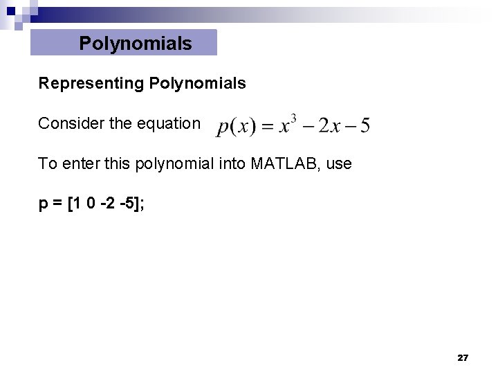
Polynomials Representing Polynomials Consider the equation To enter this polynomial into MATLAB, use p = [1 0 -2 -5]; 27

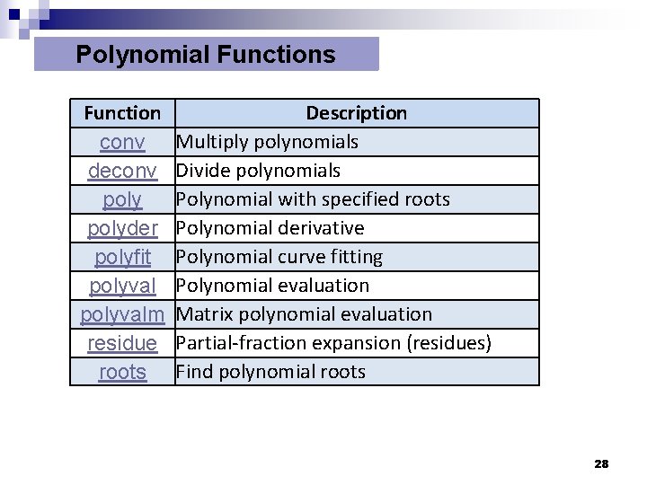
Polynomial Functions Function conv deconv polyder polyfit polyvalm residue roots Description Multiply polynomials Divide polynomials Polynomial with specified roots Polynomial derivative Polynomial curve fitting Polynomial evaluation Matrix polynomial evaluation Partial-fraction expansion (residues) Find polynomial roots 28

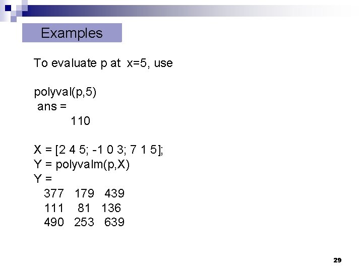
Examples To evaluate p at x=5, use polyval(p, 5) ans = 110 X = [2 4 5; -1 0 3; 7 1 5]; Y = polyvalm(p, X) Y= 377 179 439 111 81 136 490 253 639 29

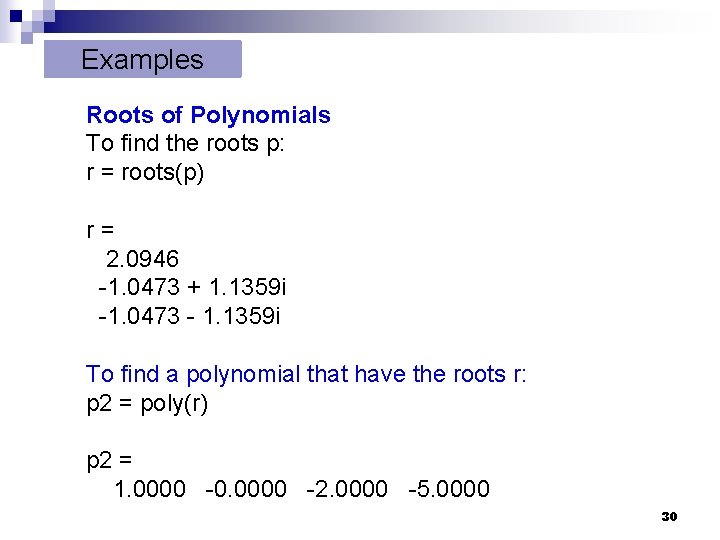
Examples Roots of Polynomials To find the roots p: r = roots(p) r= 2. 0946 -1. 0473 + 1. 1359 i -1. 0473 - 1. 1359 i To find a polynomial that have the roots r: p 2 = poly(r) p 2 = 1. 0000 -0. 0000 -2. 0000 -5. 0000 30

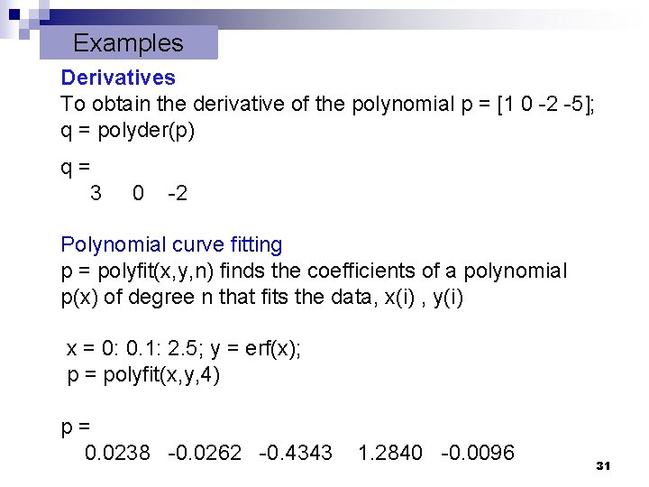
Examples Derivatives To obtain the derivative of the polynomial p = [1 0 -2 -5]; q = polyder(p) q= 3 0 -2 Polynomial curve fitting p = polyfit(x, y, n) finds the coefficients of a polynomial p(x) of degree n that fits the data, x(i) , y(i) x = 0: 0. 1: 2. 5; y = erf(x); p = polyfit(x, y, 4) p= 0. 0238 -0. 0262 -0. 4343 1. 2840 -0. 0096 31

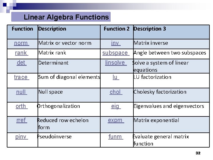
Linear Algebra Functions Function Description norm Matrix or vector norm rank Matrix rank det Determinant trace Sum of diagonal elements Function 2 Description 3 inv Matrix inverse subspace Angle between two subspaces lu Solve a system of linear equations LU factorization linsolve null Null space chol Cholesky factorization orth Orthogonalization eig Eigenvalues and eigenvectors rref Reduced row echelon form expm Matrix exponential pinv Pseudoinverse funm Evaluate general matrix function 32

Examples U= A=[1 -2 3; 4 0 6; 2 -1, 3] [L, U, P] = lu(A) A= 1 4 2 -2 0 -1 L= 1. 0000 0. 2500 0. 5000 P= 0 1 0 3 6 3 0 1. 0000 0. 5000 4. 0000 0 6. 0000 0 -2. 0000 1. 5000 0 0 -0. 7500 1 0 0 1. 0000 33

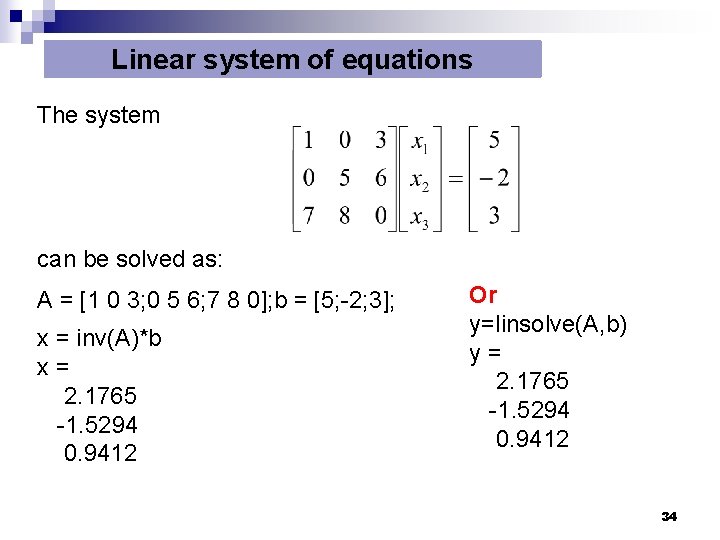
Linear system of equations The system can be solved as: A = [1 0 3; 0 5 6; 7 8 0]; b = [5; -2; 3]; x = inv(A)*b x= 2. 1765 -1. 5294 0. 9412 Or y=linsolve(A, b) y= 2. 1765 -1. 5294 0. 9412 34

Plot

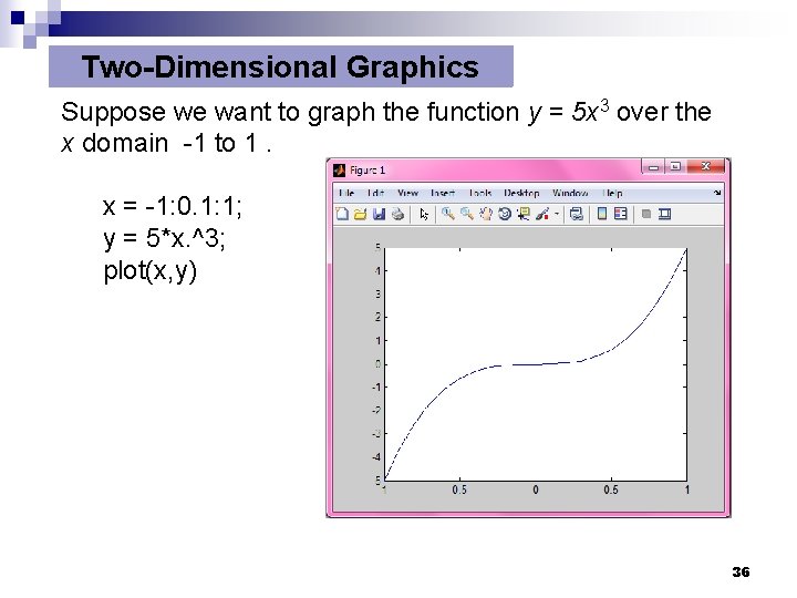
Two-Dimensional Graphics Suppose we want to graph the function y = 5 x 3 over the x domain -1 to 1. x = -1: 0. 1: 1; y = 5*x. ^3; plot(x, y) 36

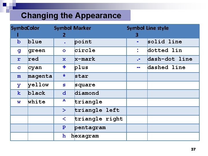
Changing the Appearance Symbo. Color Symbol Marker Symbol Line style l 2 3 b blue. point solid line g green o circle : dotted lin r red x x-mark. - dash-dot line c cyan + plus -- dashed line m magenta * star y yellow s square k black d diamond w white ^ triangle > triangle left < triangle right P pentagram h hexagram 37

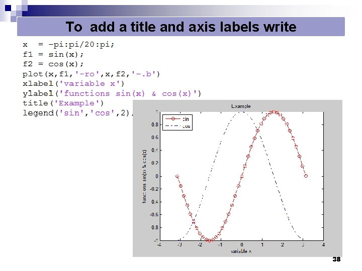
To add a title and axis labels write 38

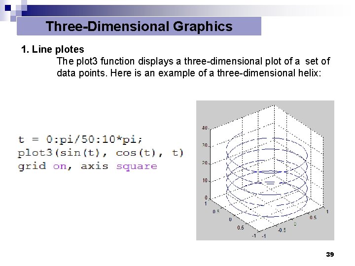
Three-Dimensional Graphics 1. Line plotes The plot 3 function displays a three-dimensional plot of a set of data points. Here is an example of a three-dimensional helix: 39

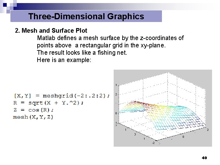
Three-Dimensional Graphics 2. Mesh and Surface Plot Matlab defines a mesh surface by the z-coordinates of points above a rectangular grid in the xy-plane. The result looks like a fishing net. Here is an example: 40

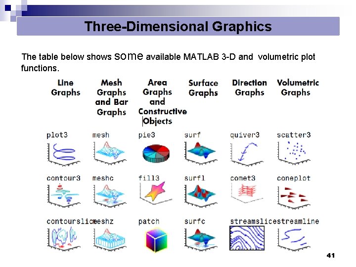
Three-Dimensional Graphics The table below shows some available MATLAB 3 -D and volumetric plot functions. 41

Symbolic Math Toolbox

Using symbolic math toolbox we can do: • • • Differentiation Integration Linear algebraic operations Simplification Transforms Variable-precision arithmetic Equation solving …………. . 43

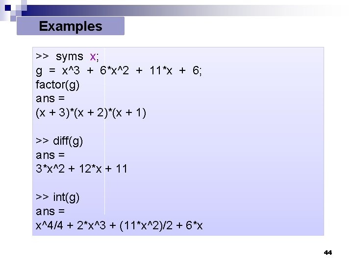
Examples >> syms x; g = x^3 + 6*x^2 + 11*x + 6; factor(g) ans = (x + 3)*(x + 2)*(x + 1) >> diff(g) ans = 3*x^2 + 12*x + 11 >> int(g) ans = x^4/4 + 2*x^3 + (11*x^2)/2 + 6*x 44

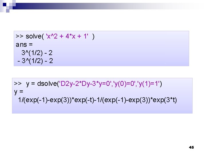
>> solve( 'x^2 + 4*x + 1' ) ans = 3^(1/2) - 2 - 3^(1/2) - 2 >> y = dsolve('D 2 y-2*Dy-3*y=0', 'y(0)=0', 'y(1)=1') y= 1/(exp(-1)-exp(3))*exp(-t)-1/(exp(-1)-exp(3))*exp(3*t) 45

Control Flow and if Statement

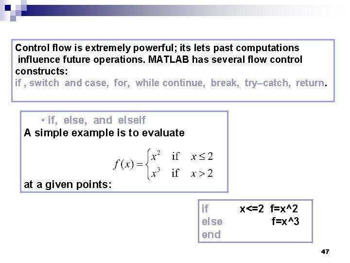
Control flow is extremely powerful; its lets past computations influence future operations. MATLAB has several flow control constructs: if , switch and case, for, while continue, break, try–catch, return. • if, else, and elseif A simple example is to evaluate at a given points: if else end x<=2 f=x^3 47

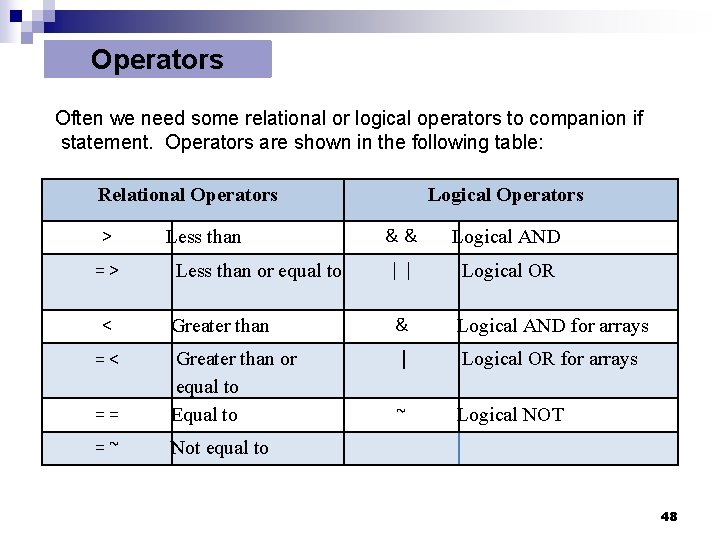
Operators Often we need some relational or logical operators to companion if statement. Operators are shown in the following table: Relational Operators > => < =< Logical Operators && Logical AND Less than or equal to || Logical OR Greater than & Logical AND for arrays | Logical OR for arrays ~ Logical NOT Less than == Greater than or equal to Equal to =~ Not equal to 48

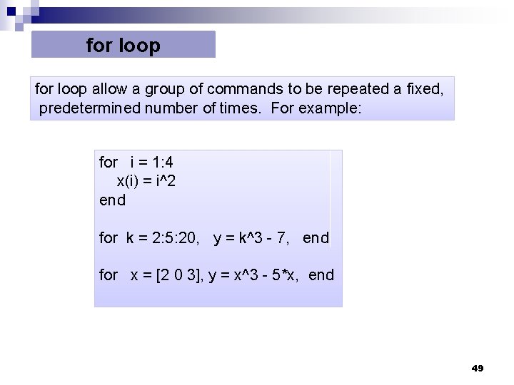
for loop allow a group of commands to be repeated a fixed, predetermined number of times. For example: for i = 1: 4 x(i) = i^2 end for k = 2: 5: 20, y = k^3 - 7, end for x = [2 0 3], y = x^3 - 5*x, end 49

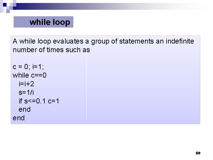
while loop A while loop evaluates a group of statements an indefinite number of times such as c = 0; i=1; while c==0 i=i+2 s=1/i if s<=0. 1 c=1 end 50

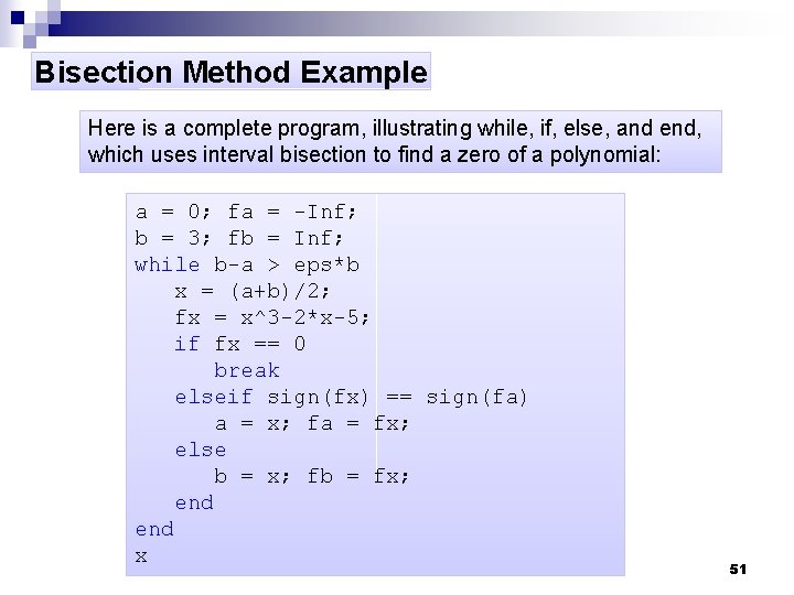
Bisection Method Example Here is a complete program, illustrating while, if, else, and end, which uses interval bisection to find a zero of a polynomial: a = 0; fa = -Inf; b = 3; fb = Inf; while b-a > eps*b x = (a+b)/2; fx = x^3 -2*x-5; if fx == 0 break elseif sign(fx) == sign(fa) a = x; fa = fx; else b = x; fb = fx; end x 51

Functions

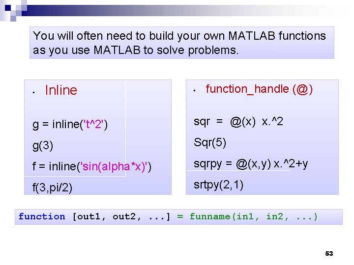
You will often need to build your own MATLAB functions as you use MATLAB to solve problems. • Inline • function_handle (@) g = inline('t^2') sqr = @(x) x. ^2 g(3) Sqr(5) f = inline('sin(alpha*x)') sqrpy = @(x, y) x. ^2+y f(3, pi/2) srtpy(2, 1) function [out 1, out 2, . . . ] = funname(in 1, in 2, . . . ) 53

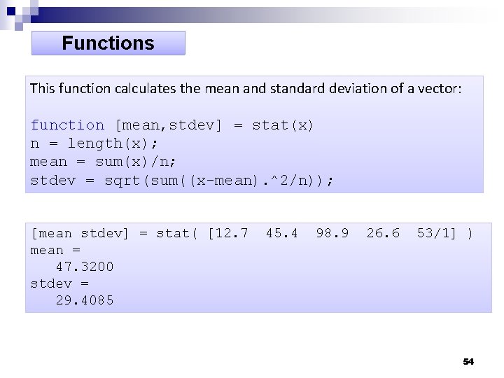
Functions This function calculates the mean and standard deviation of a vector: function [mean, stdev] = stat(x) n = length(x); mean = sum(x)/n; stdev = sqrt(sum((x-mean). ^2/n)); [mean stdev] = stat( [12. 7 mean = 47. 3200 stdev = 29. 4085 45. 4 98. 9 26. 6 53/1] ) 54

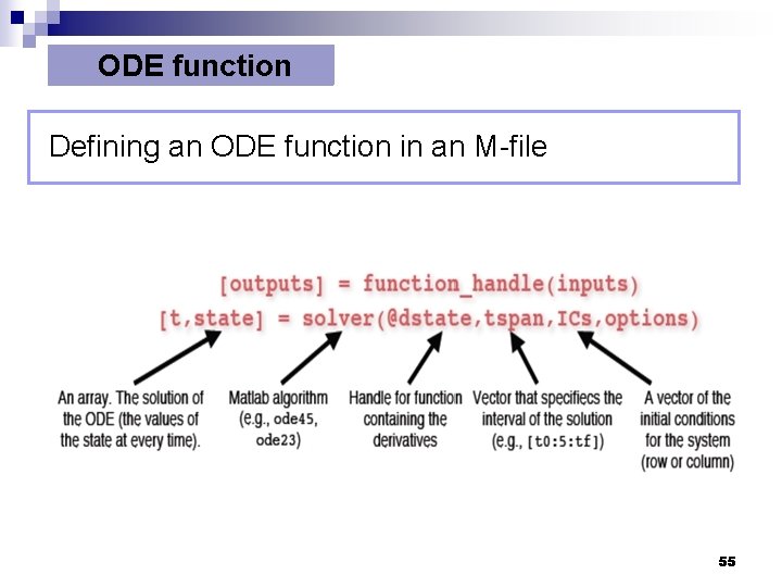
ODE function Defining an ODE function in an M-file 55

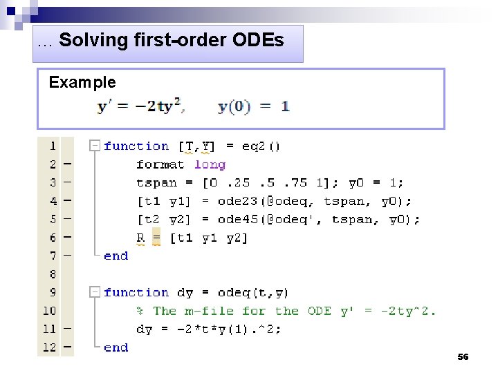
. . . Solving first-order ODEs Example 56

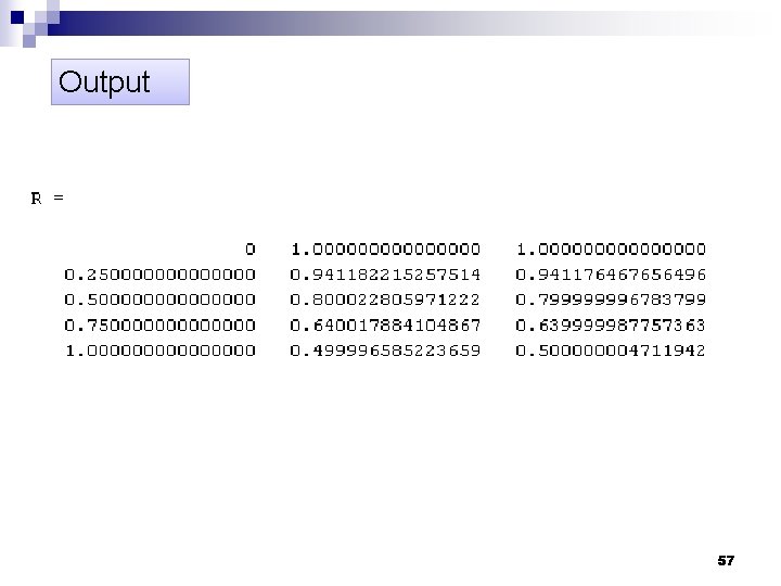
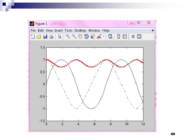
Output 57

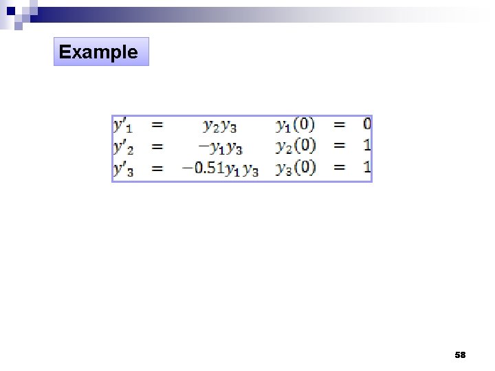
Example 58

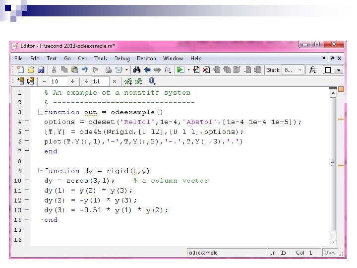
59

60

Problems

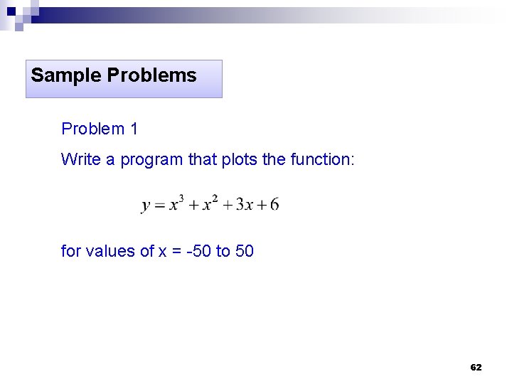
Sample Problems Problem 1 Write a program that plots the function: for values of x = -50 to 50 62

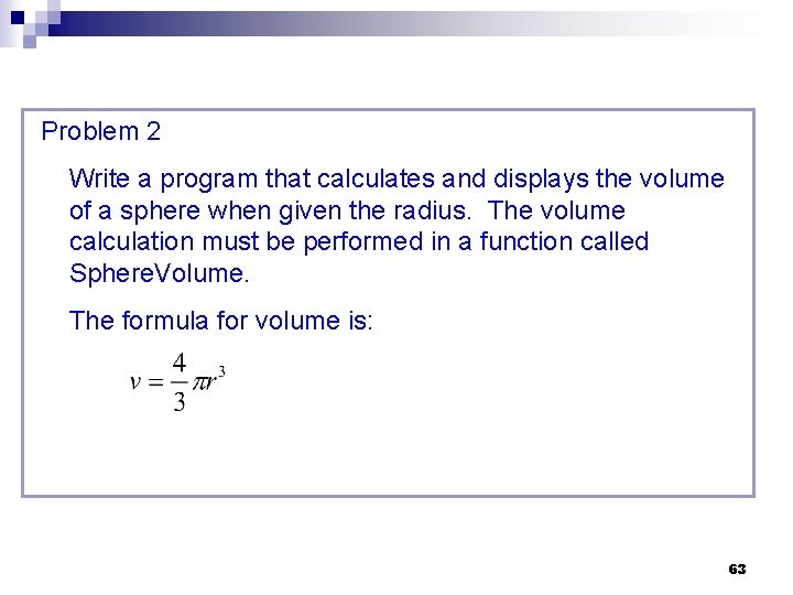
Problem 2 Write a program that calculates and displays the volume of a sphere when given the radius. The volume calculation must be performed in a function called Sphere. Volume. The formula for volume is: 63

The End