Introduction to MATLAB ES 156 Signals and Systems

Introduction to MATLAB ES 156 Signals and Systems 2007 Harvard SEAS Prepared by Jiajun Gu

Outline • Introduction and where to get MATLAB • Data structure: matrices, vectors and operations • Basic line plots • File I/O

Where to get MATLAB • FAS computing: – Download from http: //fas. harvard. edu/computing/software/ – You must be on FAS network to use MATLAB • HSEAS IT – Maxwell Dworkin Rooms G 107 -G 111 • Mathworks: – Student version is affordable and complete.

What is MATLAB • High level language for technical computing • Stands for MATrix LABoratory • Everything is a matrix - easy to do linear algebra

The MATLAB System • Development Environment • Mathematical Function Library • MATLAB language • Application Programming Language (not discussed today)

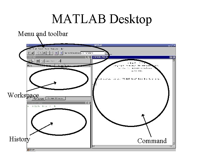
MATLAB Desktop Menu and toolbar Workspace History Command

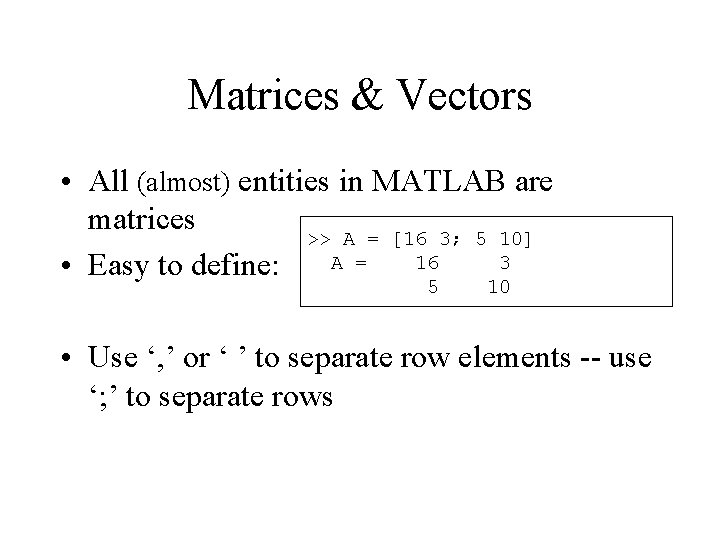
Matrices & Vectors • All (almost) entities in MATLAB are matrices >> A = [16 3; 5 10] A = 16 3 • Easy to define: 5 10 • Use ‘, ’ or ‘ ’ to separate row elements -- use ‘; ’ to separate rows

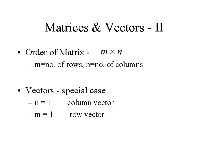
Matrices & Vectors - II • Order of Matrix – m=no. of rows, n=no. of columns • Vectors - special case –n=1 –m=1 column vector row vector

Creating Vectors and Matrices • Define >> A = [16 3; 5 10] A = 16 3 5 10 >> B = [3 4 5 6 7 8] B = 3 4 5 6 7 8 • Transpose Vector : >> a=[1 2 3]; >> a' 1 2 3 Matrix: >> A=[1 2; 3 4]; >> A' ans = 1 3 2 4

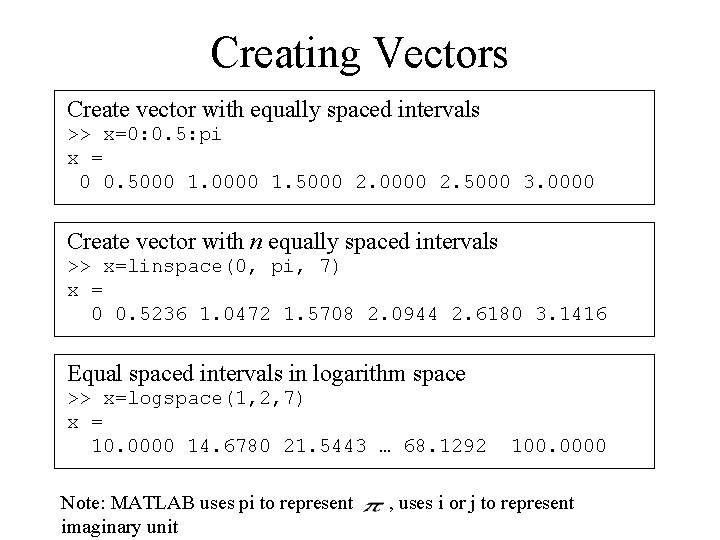
Creating Vectors Create vector with equally spaced intervals >> x=0: 0. 5: pi x = 0 0. 5000 1. 0000 1. 5000 2. 0000 2. 5000 3. 0000 Create vector with n equally spaced intervals >> x=linspace(0, pi, 7) x = 0 0. 5236 1. 0472 1. 5708 2. 0944 2. 6180 3. 1416 Equal spaced intervals in logarithm space >> x=logspace(1, 2, 7) x = 10. 0000 14. 6780 21. 5443 … 68. 1292 Note: MATLAB uses pi to represent imaginary unit 100. 0000 , uses i or j to represent

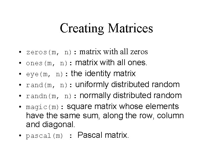
Creating Matrices • zeros(m, n): matrix with all zeros • ones(m, n): matrix with all ones. • eye(m, n): the identity matrix • rand(m, n): uniformly distributed random • randn(m, n): normally distributed random • magic(m): square matrix whose elements have the same sum, along the row, column and diagonal. • pascal(m) : Pascal matrix.

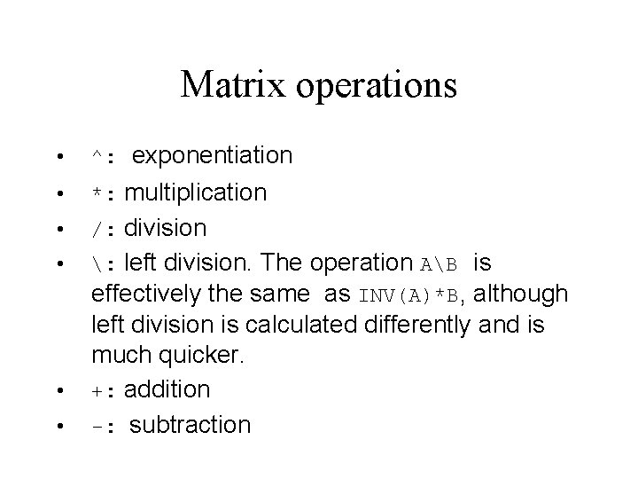
Matrix operations • ^: exponentiation • *: multiplication • /: division • : left division. The operation AB is effectively the same as INV(A)*B, although left division is calculated differently and is much quicker. • +: addition • -: subtraction

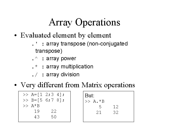
Array Operations • Evaluated element by element. ' : array transpose (non-conjugated transpose). ^ : array power. * : array multiplication. / : array division • Very different from Matrix operations >> A=[1 2; 3 4]; >> B=[5 6; 7 8]; >> A*B 19 22 43 50 But: >> A. *B 5 21 12 32

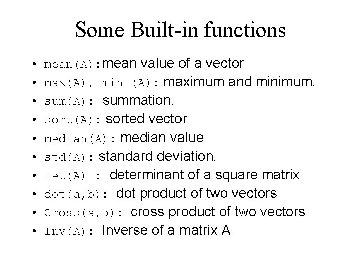
Some Built-in functions • mean(A): mean value of a vector • max(A), min (A): maximum and minimum. • sum(A): summation. • sort(A): sorted vector • median(A): median value • std(A): standard deviation. • det(A) : determinant of a square matrix • dot(a, b): dot product of two vectors • Cross(a, b): cross product of two vectors • Inv(A): Inverse of a matrix A

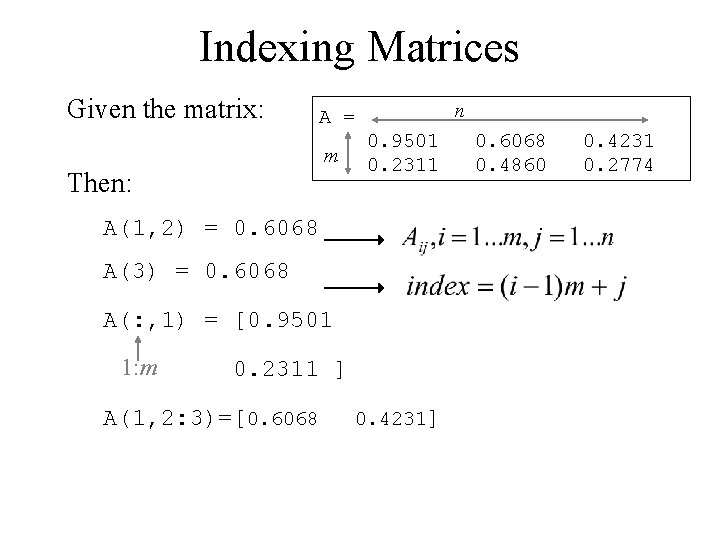
Indexing Matrices Given the matrix: n A = m Then: 0. 9501 0. 2311 A(1, 2) = 0. 6068 A(3) = 0. 6068 A(: , 1) = [0. 9501 1: m 0. 2311 ] A(1, 2: 3)=[0. 6068 0. 4231] 0. 6068 0. 4860 0. 4231 0. 2774

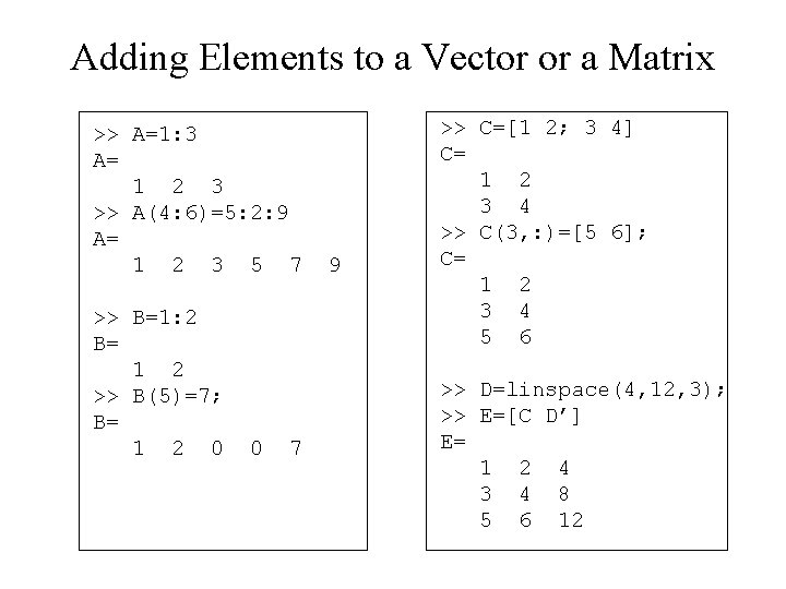
Adding Elements to a Vector or a Matrix >> A=1: 3 A= 1 2 3 >> A(4: 6)=5: 2: 9 A= 1 2 3 5 7 >> B=1: 2 B= 1 2 >> B(5)=7; B= 1 2 0 0 7 9 >> C=[1 2; 3 4] C= 1 2 3 4 >> C(3, : )=[5 6]; C= 1 2 3 4 5 6 >> D=linspace(4, 12, 3); >> E=[C D’] E= 1 2 4 3 4 8 5 6 12

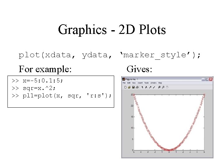
Graphics - 2 D Plots plot(xdata, ydata, ‘marker_style’); For example: >> x=-5: 0. 1: 5; >> sqr=x. ^2; >> pl 1=plot(x, sqr, 'r: s'); Gives:

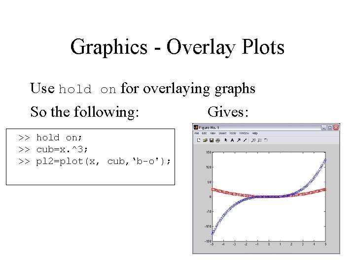
Graphics - Overlay Plots Use hold on for overlaying graphs So the following: Gives: >> hold on; >> cub=x. ^3; >> pl 2=plot(x, cub, ‘b-o');

Graphics - Annotation Use title, xlabel, annotation ylabel and legend for >> title('Demo plot'); >> xlabel('X Axis'); >> ylabel('Y Axis'); >> legend([pl 1, pl 2], 'x^2', 'x^3');

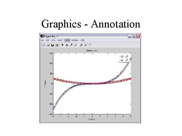
Graphics - Annotation

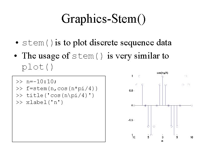
Graphics-Stem() • stem()is to plot discrete sequence data • The usage of stem() is very similar to plot() >> >> n=-10: 10; f=stem(n, cos(n*pi/4)) title('cos(npi/4)') xlabel('n')

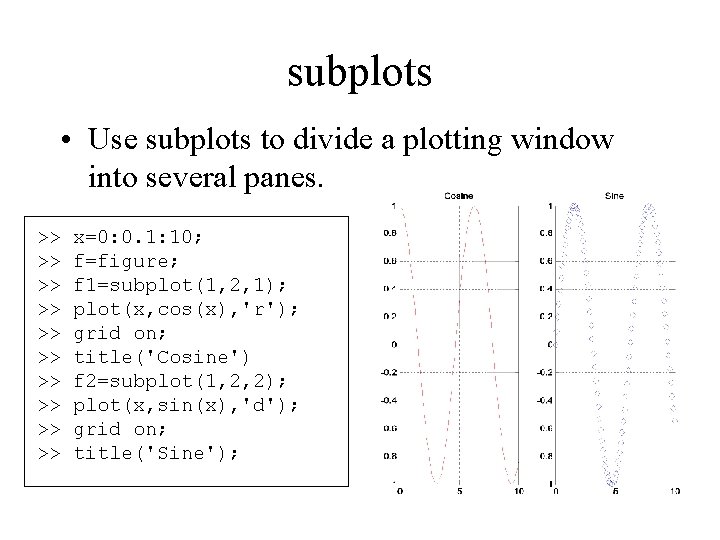
subplots • Use subplots to divide a plotting window into several panes. >> >> >> x=0: 0. 1: 10; f=figure; f 1=subplot(1, 2, 1); plot(x, cos(x), 'r'); grid on; title('Cosine') f 2=subplot(1, 2, 2); plot(x, sin(x), 'd'); grid on; title('Sine');

Save plots • Use saveas(h, 'filename. ext') to save a figure to a file. >> >> f=figure; x=-5: 0. 1: 5; h=plot(x, cos(2*x+pi/3)); title('Figure 1'); xlabel('x'); saveas(h, 'figure 1. fig') saveas(h, 'figure 1. eps') Useful extension types: bmp: Windows bitmap emf: Enhanced metafile eps: EPS Level 1 fig: MATLAB figure jpg: JPEG image m: MATLAB M-file tif: TIFF image, compressed

Workspace • • Matlab remembers old commands And variables as well Each Function maintains its own scope The keyword clear removes all variables from workspace • The keyword who lists the variables

File I/O • Matlab has a native file format to save and load workspaces. Use keywords load and save. • In addition MATLAB knows a large number of popular formats. Type “help fileformats” for a listing. • In addition MATLAB supports ‘C’ style low level file I/O. Type “help fprintf” for more information.

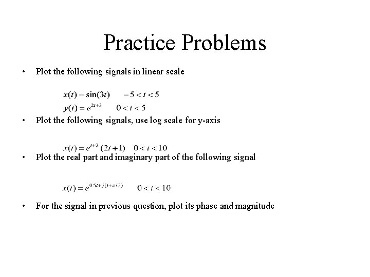
Practice Problems • Plot the following signals in linear scale • Plot the following signals, use log scale for y-axis • Plot the real part and imaginary part of the following signal • For the signal in previous question, plot its phase and magnitude