Introduction to MATLAB EE589 Introduction to Neural Networks

Introduction to MATLAB EE-589 Introduction to Neural Networks

History of MATLAB • Ancestral software to MATLAB – Fortran subroutines for solving linear (LINPACK) and eigenvalue (EISPACK) problems – Developed primarily by Cleve Moler in the 1970’s

History of MATLAB, con’t: 2 • The Mathworks, Inc. was created in 1984 • The Mathworks is now responsible for development, sale, and support for MATLAB • The Mathworks is located in Natick, MA • The Mathworks is an employer that hires co-ops through our co-op program

MATLAB GUI • Launch Pad / Toolbox • Workspace • Current Directory • Command History • Command Window

Launch Pad / Toolbox • Will not be covered • Launch Pad allows you to start help/demos • Toolbox is for use with specialized packages (Signal Processing)

Workspace • Allows access to data • Area of memory managed through the Command Window • Shows Name, Size (in elements), Number of Bytes and Type of Variable

Current Directory • MATLAB, like Windows or UNIX, has a current directory • MATLAB functions can be called from any directory • Your programs (to be discussed later) are only available if the current directory is the one that they exist in

Command History • Allows access to the commands used during this session, and possibly previous sessions • Clicking and dragging to the Command window allows you to re-execute previous commands

Command Window • Probably the most important part of the GUI • Allows you to input the commands that will create variables, modify variables and even (later) execute scripts and functions you program yourself.

Save • save – saves workspace variables on disk • save filename stores all workspace variables in the current directory in filename. mat • save filename var 1 var 2. . . saves only the specified workspace variables in filename. mat. Use the * wildcard to save only those variables that match the specified pattern.

Clear • clear removes items from workspace, freeing up system memory • Examples of syntax: – clear name 1 name 2 name 3. . .

clc • Not quite clear • clc clears only the command window, and has no effect on variables in the workspace.

Load • load - loads workspace variables from disk • Examples of Syntax: – load filename X Y Z

• The presence or lack of a semi-colon after a MATLAB command does not generate an error of any kind • The presence of a semi-colon tells MATLAB to suppress the screen output of the command

• The lack of a semi-colon will make MATLAB output the result of the command you entered • One of these options is not necessarily better than the other

Declaring a variable, con’t: 3 • You may now use the simple integer or float that you used like a normal number (though internally it is treated like a 1 by 1 matrix) • Possible operations: – +, -, / – Many functions (round(), ceil(), floor())

Declaring a variable, con’t: 4 • You may also make a vector rather simply • The syntax is to set a variable name equal to some numbers, which are surrounded by brackets and separated by either spaces or commas • Ex. A = [1 2 3 4 5]; • Or A = [1, 2, 3, 4, 5];

Declaring a variable, con’t: 5 • You may also declare a variable in a general fashion much more quickly • Ex. A = 1: 1: 10 • The first 1 would indicate the number to begin counting at • The second 1 would be the increase each time • And the count would end at 10

Declaring a variable, con’t: 6 • Matrices are the primary variable type for MATLAB • Matrices are declared similar to the declaration of a vector • Begin with a variable name, and set it equal to a set of numbers, surrounded by brackets. Each number should be seperated by a comma or semi-colon

Declaring a variable, con’t: 7 • The semi-colons in a matrix declaration indicate where the row would end • Ex. A = [ 1, 2; 3, 4] would create a matrix that looks like [12 34]

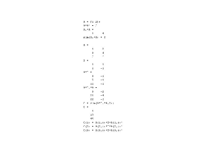
• Everything is matrix

• Matrix index

• Manipulate matrices

• Script or function? – Scripts are m-files containing MATLAB statements – Functions are like any other m-file, but they accept arguments – It is always recommended to name function file the same as the function name

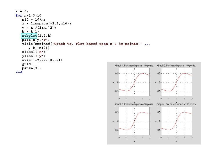
• Try to code in matrix ways

• Script m-files

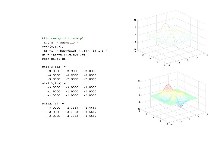
mesh

x=[ -10: 1: 10]; y = [-10: 4: 10]; [x, y] = meshgrid(x, y); z = x. ^2 + y. ^2; mesh(x, y, z); title('Mesh Ornek 3'); ylabel('Y Ekseni'); xlabel('X Ekseni'); zlabel('Z Eksen');

Plotting • Several types of plots available • • Plot Polar Bar Hist

Color options • Color options: – – – – Yellow - ‘y’ Magenta - ‘m’ Cyan - ‘c’ Red - ‘r’ Green - ‘g’ Blue - ‘b’ White - ‘w’ Black - ‘k’ • Example: • plot(temp, ‘y’);

Line options • Line styles: – - solid line (default) – -- dashed line – : dotted line – -. dash-dot line

Marker Options • • • • + - plus sign o - circle * - asterisk. - Point x - cross s - square d - diamond ^ - upward pointing triangle v - downward pointing triangle > - right pointing triangle < - left pointing triangle p - five-pointed star (pentagram) h - six-pointed star (hexagram)

Plot() (from MATLAB help) • Linear 2 -D plot • Syntax: – plot(Y) – plot(X 1, Y 1, . . . ) – plot(X 1, Y 1, Line. Spec, . . . ) – plot(. . . , 'Property. Name', Property. Value, . . . ) – h = plot(. . . )

Plot() con’t: 2 • MATLAB defaults to plotting a blue line between points • Other options exist: – Different color lines – Different types of lines – No line at all!

Example angle = linspace(0, 2*pi, 360); x = cos(angle); y = sin(angle); plot(x, y); % it draws a circle axis('equal'); ylabel('y'); xlabel('x'); title('Pretty Circle') ; grid on

Polar() • Plot polar coordinates • Syntax: – polar(theta, rho) – polar(theta, rho, Line. Spec) • Theta – Angle counterclockwise from the 3 o’clock position • Rho – Distance from the origin

Polar() con’t: 2 • Line color, style and markings apply as they did in the example with Plot(). t = 0: . 01: 2*pi; polar(t, sin(2*t). *cos(2*t), '--r')

Bar() • Creates a bar graph • Syntax – bar(Y) – bar(x, Y) – bar(. . . , width) – bar(. . . , 'style') – bar(. . . , Line. Spec)

Bar example subplot(3, 1, 1), bar(rand(10, 5), 'stacked'), colormap(cool) subplot(3, 1, 2), bar(0: . 25: 1, rand(5), 1) subplot(3, 1, 3), bar(rand(2, 3), . 75, 'grouped')

Hist() • Creates a histogram plot • Syntax: – n = hist(Y) – n = hist(Y, x) – n = hist(Y, nbins) Example x = -4: 0. 1: 4; y = randn(10000, 1); hist(y, x)

Pie x=[. 19. 22. 41. 18]; pie(x) explode = zeros(size(x)); h = pie(x, explode); text. Objs = findobj(h, 'Type', 'text'); old. Str = get(text. Objs, {'String'}); val = get(text. Objs, {'Extent'}); old. Ext = cat(1, val{: }); Names = {'P 1: '; 'P 2: '; 'P 3: '; 'P 4: '}; new. Str = strcat(Names, old. Str); set (text. Objs, {'String'}, new. Str)

Another satisfied MATLAB user! End