Introduction to MATLAB Basics Solving quadratic formula Fibonacci

Introduction to MATLAB Basics Solving quadratic formula Fibonacci Series Magic Squares SCV-ASU 1

The MATLAB Desktop SCV-ASU 2

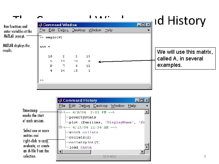
The Command Window and History We will use this matrix, called A, in several examples. SCV-ASU 3

The Help System SCV-ASU 4

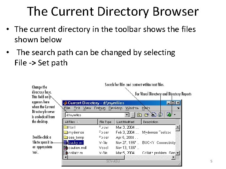
The Current Directory Browser • The current directory in the toolbar shows the files shown below • The search path can be changed by selecting File -> Set path SCV-ASU 5

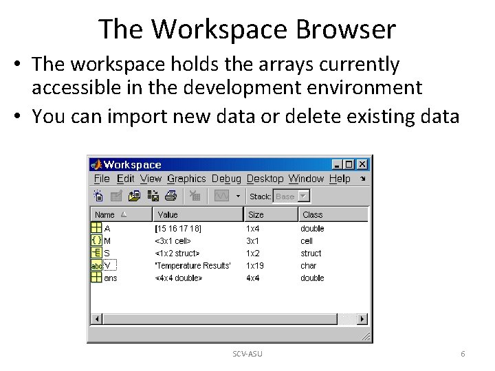
The Workspace Browser • The workspace holds the arrays currently accessible in the development environment • You can import new data or delete existing data SCV-ASU 6

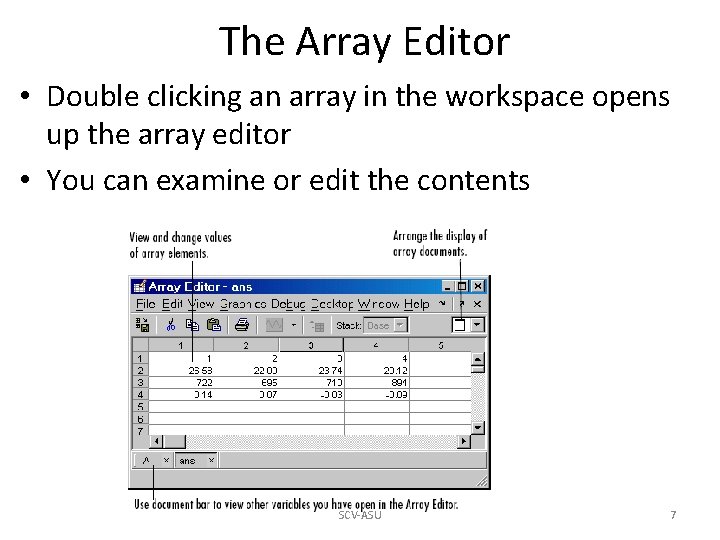
The Array Editor • Double clicking an array in the workspace opens up the array editor • You can examine or edit the contents SCV-ASU 7

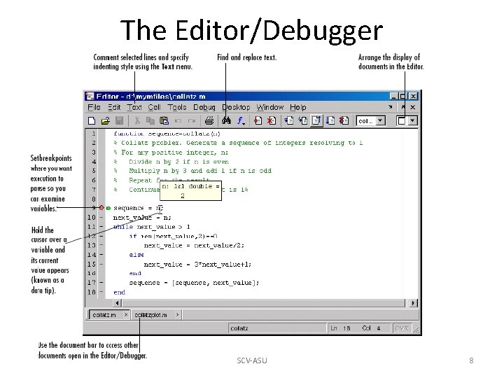
The Editor/Debugger SCV-ASU 8

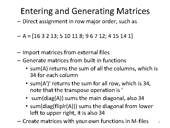
Entering and Generating Matrices – Direct assignment in row major order, such as – A = [16 3 2 13; 5 10 11 8; 9 6 7 12; 4 15 14 1] – Import matrices from external files – Generate matrices from built-in functions • sum(A) returns the sum of all the columns, which is 34 for each column • sum(A′)′ returns the sum for all row, which is 34, note that the transpose operation is ′ • sum(diag(A)) sums the main diagonal, also 34 • sum(diag(fliplr(A))) sums the diagonal from lower left to upper right, it is also 34 – Create matrices with your own functions in M-files SCV-ASU 9

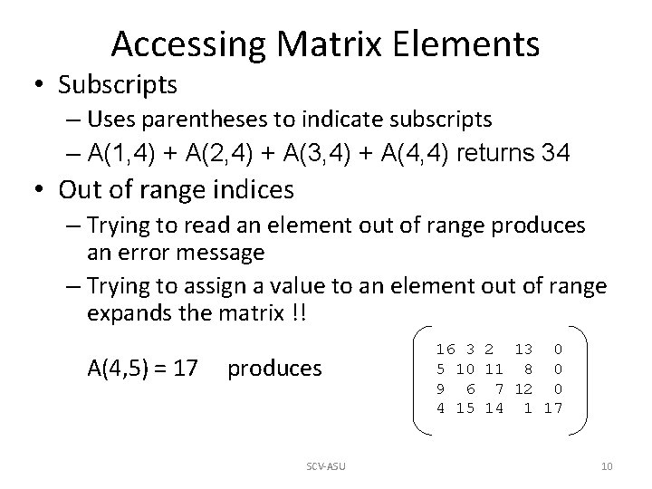
Accessing Matrix Elements • Subscripts – Uses parentheses to indicate subscripts – A(1, 4) + A(2, 4) + A(3, 4) + A(4, 4) returns 34 • Out of range indices – Trying to read an element out of range produces an error message – Trying to assign a value to an element out of range expands the matrix !! A(4, 5) = 17 produces SCV-ASU 16 3 2 13 0 5 10 11 8 0 9 6 7 12 0 4 15 14 1 17 10

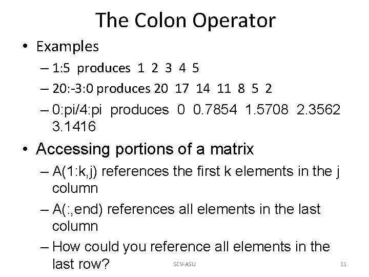
The Colon Operator • Examples – 1: 5 produces 1 2 3 4 5 – 20: -3: 0 produces 20 17 14 11 8 5 2 – 0: pi/4: pi produces 0 0. 7854 1. 5708 2. 3562 3. 1416 • Accessing portions of a matrix – A(1: k, j) references the first k elements in the j column – A(: , end) references all elements in the last column – How could you reference all elements in the SCV-ASU 11 last row?

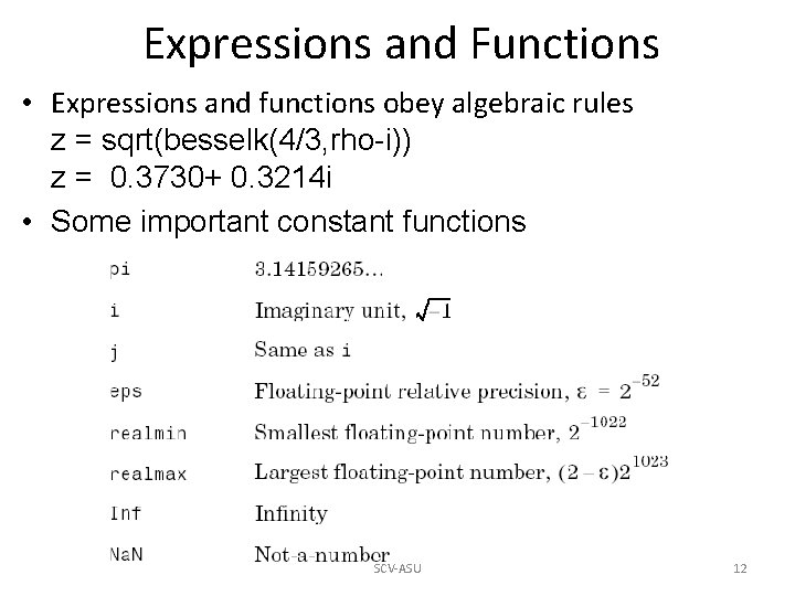
Expressions and Functions • Expressions and functions obey algebraic rules z = sqrt(besselk(4/3, rho-i)) z = 0. 3730+ 0. 3214 i • Some important constant functions SCV-ASU 12

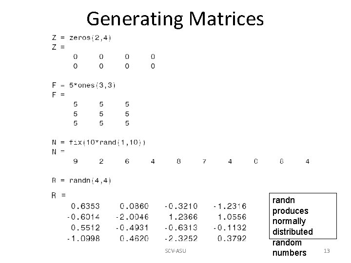
Generating Matrices SCV-ASU randn produces normally distributed random numbers 13

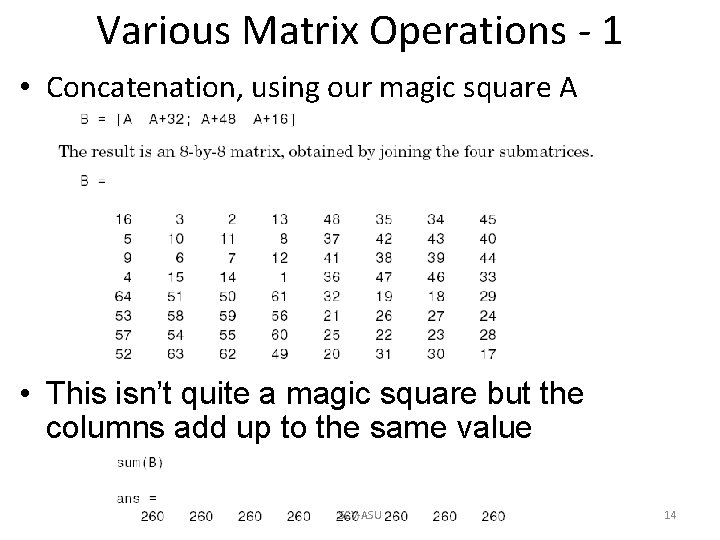
Various Matrix Operations - 1 • Concatenation, using our magic square A • This isn’t quite a magic square but the columns add up to the same value SCV-ASU 14

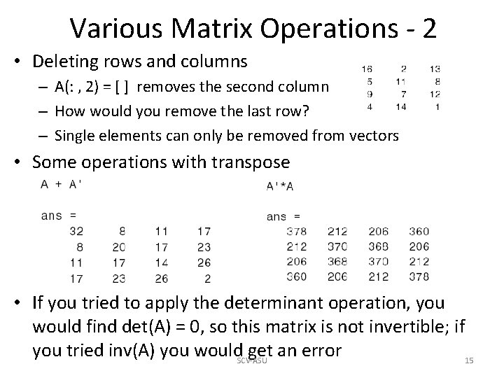
Various Matrix Operations - 2 • Deleting rows and columns – A(: , 2) = [ ] removes the second column – How would you remove the last row? – Single elements can only be removed from vectors • Some operations with transpose • If you tried to apply the determinant operation, you would find det(A) = 0, so this matrix is not invertible; if you tried inv(A) you would. SCV-ASU get an error 15

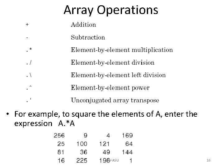
Array Operations • For example, to square the elements of A, enter the expression A. *A SCV-ASU 16

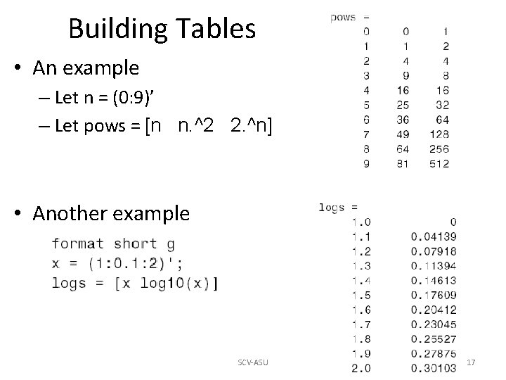
Building Tables • An example – Let n = (0: 9)’ – Let pows = [n n. ^2 2. ^n] • Another example SCV-ASU 17

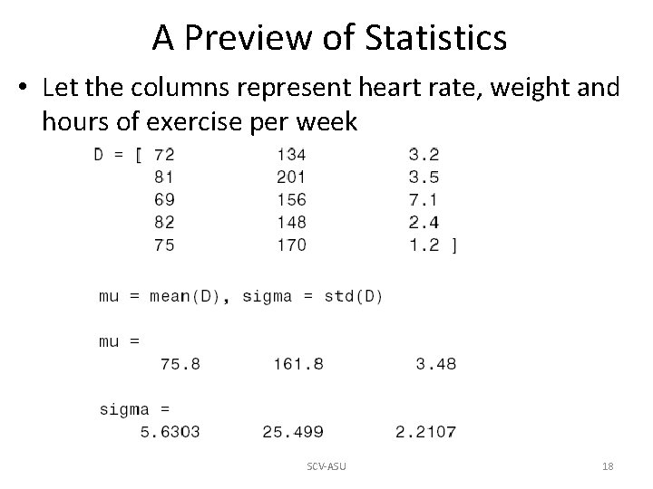
A Preview of Statistics • Let the columns represent heart rate, weight and hours of exercise per week SCV-ASU 18

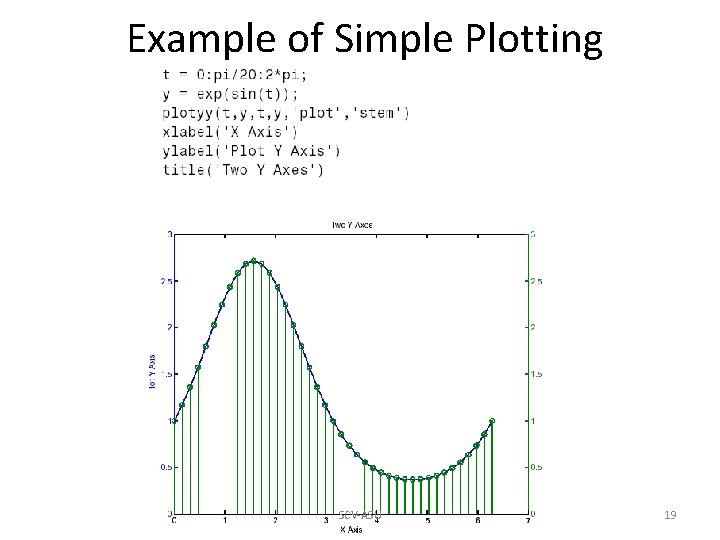
Example of Simple Plotting SCV-ASU 19

An Example - 1 x = -1: . 1: 1; % Define the range of x y = x. ^3; % Raise each element in x to the third power plottools SCV-ASU 20

An Example - 2 SCV-ASU 21

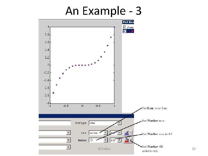
An Example - 3 SCV-ASU 22

Programming in MATLAB • Control structures – Selection (if and switch) – Repetition (for, while, break, continue) • • Dynamic Structures Scripts and M files User defined functions Examples – Finding the periodicity of sunspots SCV-ASU 23

The if command • An example • Some useful boolean tests Useful Boolean tests for matrices SCV-ASU 24

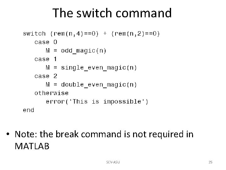
The switch command • Note: the break command is not required in MATLAB SCV-ASU 25

Commands for repetition • The for command (notice the required ‘end’) • The while command (also requires ‘end’) Does anyone recognize what this code fragment does? SCV-ASU 26

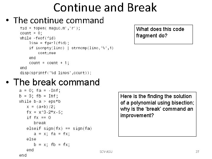
Continue and Break • The continue command What does this code fragment do? • The break command Here is the finding the solution of a polynomial using bisection; why is the ‘break’ command an improvement? SCV-ASU 27

Scripts and M files • An M file (. m extension) stores MATLAB code – The file name is used to reference the code – The code is a sequence of commands that is executed • An example Stored in magicrank. m Executed by ‘magicrank’ on command line SCV-ASU 28

Functions in MATLAB • Built-in functions – Found in toolbox/matlab/matfun – An example, the function rank SCV-ASU 29

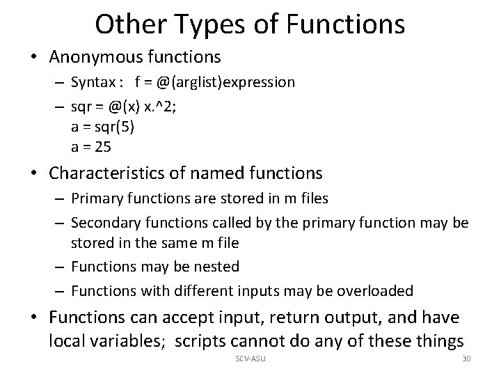
Other Types of Functions • Anonymous functions – Syntax : f = @(arglist)expression – sqr = @(x) x. ^2; a = sqr(5) a = 25 • Characteristics of named functions – Primary functions are stored in m files – Secondary functions called by the primary function may be stored in the same m file – Functions may be nested – Functions with different inputs may be overloaded • Functions can accept input, return output, and have local variables; scripts cannot do any of these things SCV-ASU 30

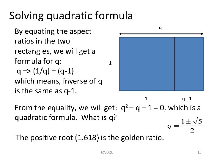
Solving quadratic formula By equating the aspect ratios in the two rectangles, we will get a formula for q: q => (1/q) = (q-1) which means, inverse of q is the same as q-1. q 1 1 q-1 From the equality, we will get: q 2 – q – 1 = 0, which is a quadratic formula. What is q? The positive root (1. 618) is the golden ratio. SCV-ASU 31

How this is done in MATLAB The coefficients in the quadratic formula: q 2 – q – 1 = 0, are c = [1 -1 -1] that correspond to the power 2, 1, and 0 of q in this formula. The roots are computed as: > R = roots(c) i. e. -0. 618 and 1. 618 We could use a function f(x) = 1/x – (x – 1) to study this a little differently: Øf = @(x) 1. /x – (x – 1) If we plot this function in a interval where there are roots, we can find that f is 0 at the root values. > ezplot(f, -1, 2); SCV-ASU 32

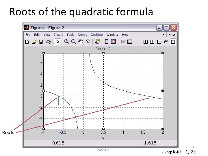
Roots of the quadratic formula Roots -0. 618 1. 618 SCV-ASU 33 > ezplot(f, -1, 2);

Fibonacci Series Here is a nice problem. I hope someone can implement this in Net. Logo. Someone put a pair of rabbits in a isolated cage. These rabbits can produce one new pair every month, and the new pair can start producing once they are 2 month or older. How many rabbits will have after a year? The answer is the 12 th Fibinacci’s number. The question we may have is, whether this series will reach a constant ratio. SCV-ASU 34

Fibonacci Series Ok, the Fibonacci Series can be written as: f(k) = f(k-1) + f(k-2) And the ratio of the two consecutive terms is: pk = f(k+1) / f(k) The question: is there is a limit to this. i. e. , will this ratio converge to a constant value? When I heard this I thought, eventually this ratio will become 2. Here is what I have generated with MATLAB. SCV-ASU 35

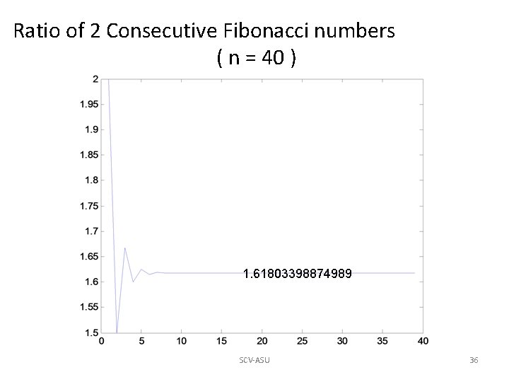
Ratio of 2 Consecutive Fibonacci numbers ( n = 40 ) 1. 61803398874989 SCV-ASU 36

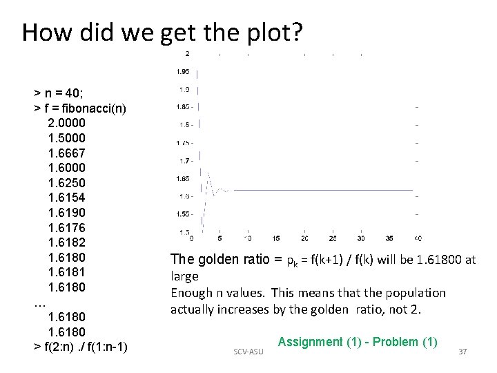
How did we get the plot? > n = 40; > f = fibonacci(n) 2. 0000 1. 5000 1. 6667 1. 6000 1. 6250 1. 6154 1. 6190 1. 6176 1. 6182 1. 6180 1. 6181 1. 6180 … 1. 6180 > f(2: n). / f(1: n-1) The golden ratio = pk = f(k+1) / f(k) will be 1. 61800 at large Enough n values. This means that the population actually increases by the golden ratio, not 2. SCV-ASU Assignment (1) - Problem (1) 37

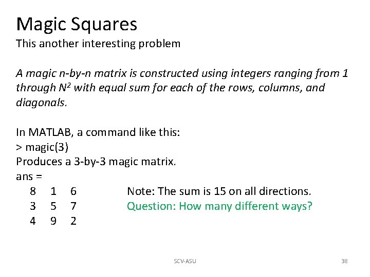
Magic Squares This another interesting problem A magic n-by-n matrix is constructed using integers ranging from 1 through N 2 with equal sum for each of the rows, columns, and diagonals. In MATLAB, a command like this: > magic(3) Produces a 3 -by-3 magic matrix. ans = 8 1 6 Note: The sum is 15 on all directions. 3 5 7 Question: How many different ways? 4 9 2 SCV-ASU 38

Question: How many different ways can we write the previous matrix? SCV-ASU 39