Introduction to MATLAB 2019 MATLAB Summer Workshop Speaker

Introduction to MATLAB© 2019 MATLAB Summer Workshop Speaker: Naomi SAWAKI (澤木直美) Email: r 07524115@ntu. edu. tw Date: 3 Sep 2019 PSE Laboratory Department of Chemical Engineering National Taiwan University PSE LABORATORY

Outline 1 1 Introduction to MATLAB© 2 Basic Operations with MATLAB 3 Use of m. files 4 Flow-Control Statements Problems (p. 52, 79~) 5 Plotting and Graphing Supplemental Materials (p. 98~) 6 Symbolic Calculation 7 Curve Fitting – Regression 8 Summary (~p. 97) PSE LABORATORY

1. Introduction Computer Languages 2 Ø MATLAB is supported by: ASCII : American Standard Code for Information Interchange BIG 5 : Chinese character encoding method (require more than 128) Example: >> abs(‘Mat. Lab’) 77 97 116 76 97 98 >> abs(‘(1~524)’) 40 49 126 53 50 52 41 >> chinese = '化學 程'; >> abs(chinese) ans = 21270 23416 24037 31243 PSE LABORATORY

1. Introduction What is interface? You Example: clear; clc; a = 4; b = 7; c = 2. 5; x = [-b + sqrt(b^2 - 4*a*c) ]/(2*a) 3 Number Systems: Ø Base 10 (Decimal) — 10 digits [0– 9] Ø Base 2 (Binary) — 2 digits [0– 1] Ex) 10101 (binary) = 24 1 + 23 0 + 22 1 + 21 0 + 20 1 = 21 (decimal) Ø Base 8 (Octal) — 8 digits [0– 7] Ex) 012 (octal) = 8 2 0 + 81 1 + 80 2 = 10 (decimal) = 1010 (binary) Ø Base 16 (Hexadecimal) — 10 digits + 6 characters [0– 9, A, B, C, D, E, F] Ex) 5 B (octal) = 162 0 + 161 5 + 160 11 = 91 (decimal) Computer Calculations Interface x = [-b + sqrt(b^2 -4*a*c) ]/(2*a) PSE LABORATORY

1. Introduction World Computer Languages 4 Ø MATLAB is one of the top 15 computer languages. Source: TIOBE Index, Top Computer Languages, Statistics Times (17 May 2019) PSE LABORATORY

1. Introduction What is MATLAB? 5 Ø MATLAB is a commercial software of Math. Works corporation 應用領域 Ø高科技運算程式解決方案 Technical Computing Ø控制設計 Control Design Ø訊號處理及通訊 Signal Processing and Communications Ø影像處理 Image Processing Ø測試及量測 Test Measurement Ø生物運算 Computational Biology Ø財務模型及分析 Financial Modeling and Analysis Ø教育專區 Education PSE LABORATORY

1. Introduction What is MATLAB? 6 ØWhat is MATLAB? – MATrix MAT LABoratory LAB – 以矩陣為運算基礎的直譯式數學程式語言 – 提供完備的數學函數, 使用者能定義自己 的函數 – 提供矩陣運算、數值分析、統計分析、訊 號處理、圖形繪製(2 D/3 D)…等功能 ØHistory of MATLAB – Prof. Cleve Moler wrote a free software MATLAB using ‘FORTRAN’ in 1978 – Jack Little rewrote Matlab with “C” and founded Math. Works in 1984. PSE LABORATORY

1. Introduction 台大虛擬桌面 8 Student number Password PSE LABORATORY

1. Introduction 台大虛擬桌面 9 Choose one virtual desktop of your choice Notes: 1. Require an internet connection. 2. Your saved files can only be found in the same virtual desktop. PSE LABORATORY

2. Basic Operation with MATLAB 10 1. MATLAB Interface 2. Special Characters 3. Useful Commands 4. Mathematical Operators 5. Rational Operators 6. Logical Operators 7. Order of Precedence 8. Matric Operations 9. 常見特殊矩陣 10. Useful Array Functions 11. 矩陣的基本資料結構 12. 變數命名規則與使用 13. 作空間與變數的儲存及載入 14. MATLAB – Excel Processing PSE LABORATORY

2. Basic Operations MATLAB R 2015 b Interface Current Folder Command Window >> clear % clear workspace >> clc % clear command window Details *Clear workspace and command window before running a new file to avoid miscalculations. ***Learn to use “help” >> help abs % matlab returns what abs function is 11 Workspace Command History PSE LABORATORY

2. Basic Operations MATLAB R 2015 b Interface 12 開啟Editor PSE LABORATORY

2. Basic Operations Special Characters Command 13 Description , Comma; separates elements of an array (元素分隔符號) ; Semicolon; suppresses screen printing; also denotes a new row in an array (代表命令結束，且不印出執行結果) : Colon; generates an array having regularly spaced elements (Ex) x = 1: 2: 10 means x = 1, 3, 5, 7, 9 % Comments (註解列) ' =. . . Assignment (指定運算) (Ex) B = A means let B be A Ellipsis; continues a line to delay execution (繼續，代表指令未完，接到下一列) PSE LABORATORY

2. Basic Operations Useful Commands Examples: Removes all variables from memory >> M = 10; N = 5; >> clear M % clear only M >> format short % 1. short >> pi ans = 3. 1416 >> format long % 2. long >> pi ans = 3. 141592653589793 >> format loose % 3. loose >> exp(2) Removes var 1 and var 2 from workspace ans = Command bench 14 Description MATLAB Benchmark cla Clear axis clc Clear command window cd Change current working directory. clf Clear figure clear var 1 var 2 dir exist(‘name’) format iskeyword quit version whos List directory Determine if a file or variable called ‘name’ exists Set command window output display format Determine whether input is MATLAB keyword Quit MATLAB session Version information for MATLAB and libraries 7. 389056098930650 >> format compact % 4. compact >> log(10) ans = 2. 302585092994046 Lists all the variables as in “who” with their size, bytes, class, etc. PSE LABORATORY

2. Basic Operations Mathematical Operators 15 Symbol Operation MATLAB Form ^ exponentiation: ab a^b * multiplication: ab a*b / a/b ab + addition: a + b a+b - subtraction: a – b a-b Examples: >> (5*2 + 3. 5)/5 ans = 2. 7000 >> 4. 2 -2^(1/2) ans = 2. 7858 For more information: https: //www. mathworks. com/help/ matlab/matlab_prog/matlaboperators-and-specialcharacters. html PSE LABORATORY

2. Basic Operations Relational Operators 16 Relational Operator < <= > Meaning Less than or equal to Greater than >= Greater than or equal to == Equal to ~= Not equal to Example: >> x = [ 6, 3, 9]; >> y = [14, 2, 9]; >> z = (x < y) z= 1 0 0 % 1 = true, 0 = false PSE LABORATORY

2. Basic Operations Logical Operator Example: Meaning & Element-wise AND | Element-wise OR && 17 Short –circuit AND || Short –circuit OR ~ Logical not any Determine if any one of array elements are nonzero or true (任何一 個元素不為 0) all Determine if all array elements are nonzero or true (所有元素都不為 0) *If you use short-circut operators, matlab calculation stops at X(2)==1 && X(4) == 3 | and X(4) == 4 is not calculated because answer is clear by the first step. >> X=[0 1 2 3] X= 0 1 2 3 >> any(X) ans = 1 >> all(X) ans = 0 >> any(X==4) ans = 0 >> X(2)==1 & X(4) == 4 ans = 0 >> X(2)==1 | X(4) == 4 ans = 1 >> X(2)==1 & X(4) == 3 ans = 1 >> X(2)==1 && X(4) == 3 | X(4) == 4 ans = 1 PSE LABORATORY

2. Basic Operations Order of Precedence 18 Precedence Operation 1 Parentheses ( ) 2 Transpose (. '), ('), power (. ^), (^) 3 Unary calculations (. ^-), (. ^+), (. ^~), (^~) 4 Unary plus (+), unary minus (-), logical negation (~) 5 Multiplication (. *), (*), division (. /), (. ), () 6 Addition (+), subtraction (-) 7 Colon operator (: ) 8 (<), (<=), (>=), (==), not equal to (~=) Example: >> 5^2*2 ans = 50 >> 5*2^2 ans = 20 >> (5*2)^2 ans = 100 PSE LABORATORY

2. Basic Operations Matrix Operations Symbol Operation 19 Form Example + Scalar-array addition A+b [6, 3]+ 2 =[8, 5] - Scalar-array subtraction A-b [6, 3]- 2 =[4, 1] + Array addition A+B [6, 3]+[3, 8] =[9, 11] - Array subtraction A-B [6, 3]-[3, 8] =[3, -5] * Matrix multiplication C*D [1, 2]*[3, 4]' =[11] Matrix left division x=C-1 E CE [1, 2][10] =[0 5]' . * Array multiplication F. *G [3, 2]. *[2, 4] =[6, 8] . / Array right division H. /G [4, 8]. /[2, 4] =[2, 2] . Array left division G. H [2, 4]. [4, 8] =[2, 2] K. ^b [3, 5]. ^2 =[9, 25] b. ^K 2. ^[3, 5] =[8, 32] F. ^L [3, 2]. ^[2, 3] =[9, 8] . ^ Array exponent Define: A = [6, 3]; b = 2; B = [3, 8]; C = [1, 2]; D = [3, 4] E = [10]; F = [3, 2]; G = [2, 4]; H = [4, 8]; K = [3, 5]; L = [2, 3]; >> [1, 2] ans = 1. 00 2. 00 >> [3, 4]' ans = 3. 00 4. 00 PSE LABORATORY

2. Basic Operations 常見特殊矩陣 Description Command [] eye(n, m) diag(A) 20 Example: 空矩陣 維度為 n x m 的identity矩陣 (usually n=m) 矩陣A的對角矩陣 linspace(x 1, x 2, n) 產生線性的空間向量 (Take n points in between x 1 and x 2) magic(n) 維度為 n x n , 元素全為整數, (Equal row, column, diagonal sums) ones(m, n) 維度為 m x n , 元素全為 1的矩陣 rand(m, n) 維度為 m x n , 於[0, 1]均勻分佈的亂數矩陣 randn(m, n) 維度為 m x n , 於[0, 1]高斯分佈的亂數矩陣 zeros(m, n) 維度為 m x n , 元素全為 0的矩陣 >> A = magic(4) A= 16 2 3 13 5 11 10 8 9 7 6 12 4 14 15 1 >> diag(A) ans = 16 11 6 1 >> eye(3) ans = 1 0 0 0 1 >> linspace(1, 10, 4) ans = 1 4 7 10 PSE LABORATORY

2. Basic Operations Useful Array Functions Command Description det(A) Return the determinant of the square matrix A eig(A) Returns a vector of the eigenvalues of matrix A find(x) Find x in an array or a matrix inv(A) Return the inverse of the square matrix A length(A) Return the number of elements of a vector A or the largest value of m or n if A is an m × n matrix max(A) Returns a row vector containing largest element in each column of A min(A) Same as max(A) but returns minimum values reshape(A) reshape(X, M, N) = reshape(X, [M, N]) returns the M-by-N matrix of X which was N-by-M matrix. size(A) Returns the sizes of the m × n array sort(A) Sorts each column of array A in ascending order sum(A) Sums the elements in each column of array A 21 Example: >> A = rand(3, 3) A= 0. 6991 0. 5472 0. 2575 0. 8909 0. 1386 0. 8407 0. 9593 0. 1493 0. 2543 >> max(A) ans = 0. 9593 0. 5472 0. 8407 >> B = [3, 8; 2, 4] B= 3 8 2 4 >> max(B) ans = 3 8 >> find(B==8) ans = 3 >> x = linspace(1, 95, 100); >> max(x) ans = 95 PSE LABORATORY

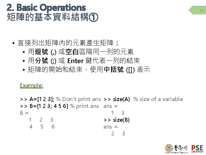
2. Basic Operations 矩陣的基本資料結構② 23 • 直接列出矩陣內的元素產生矩陣： • 或使用下列描述法構成： X = 起始值：增加值：結束值 Example: >> x 1 = 1: 10 x 1 = 1 2 3 4 5 6 >> x 2 = 1: 2: 10 x 2 = 1 3 5 7 9 >> x 3 = linspace(1, 10, 4) x 3 = 1 4 7 10 7 8 9 10 >> x 4 = linspace(0, 10) x 4 = 0 1. 1111 2. 2222 3. 3333 4. 4444 5. 5556 6. 6667 7. 7778 8. 8889 10. 0000 >> x 5 = 0: 10 x 5 = 0 1 2 9 10 3 4 5 6 7 8 % linspace can fix the number of variables. PSE LABORATORY

2. Basic Operations 矩陣的基本資料結構③ 24 Ø 矩陣的索引或下標 第九章矩陣的處理與運 Available from: http: //www. cs. nthu. edu. tw/~jang [30 July 2018] PSE LABORATORY

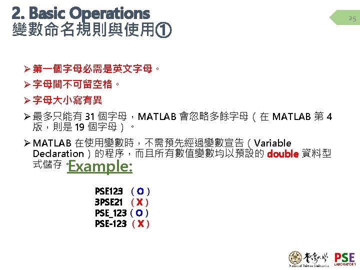
2. Basic Operations 變數命名規則與使用② 26 Ø DON’T use predefined constants as your variable names. Command Description ans Temporary variable containing the most recent answer eps Specifies the accuracy of floating point precision i, j Infinity, ∞ Na. N Indicates an undefined numerical result (Not a Number) pi The number π PSE LABORATORY

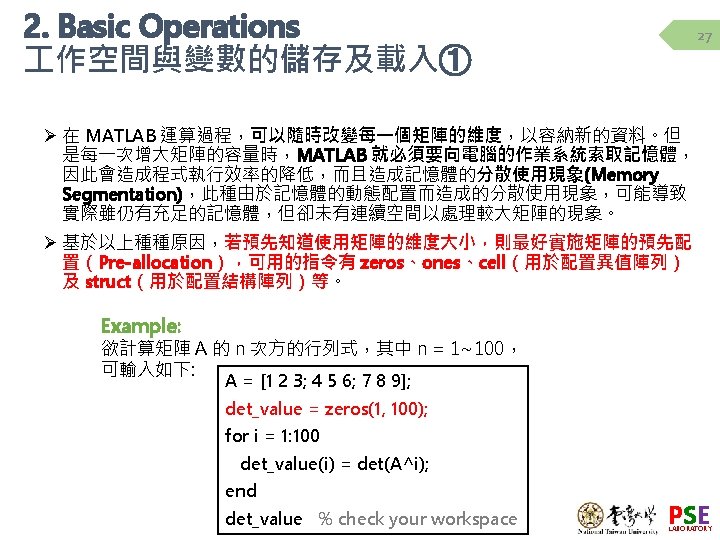
2. Basic Operations MATAB – Excel Processing 29 Your Excel file and Matlab file must be in the same folder! Ø MATAB – Excel Processing xlsfinfo: determine if file contains 而Matlab和Excel整合最大的好處，就是資 Microsoft Excel spreadsheet (讀出一個 料可以互通，因此可以輕易使用Matlab來 已存在的Excel 檔案相關資訊及裡面的 分析和畫圖處理Excel的資料。Excel也可以 作表(Sheets)名稱) 對Matlab的資料進行作圖或處理。 指令格式如下： >> xls. File = 'ROPX-economics. xlsx'; >> [file. Type, sheets] = xlsfinfo(xls. File) file. Type = Microsoft Excel Spreadsheets = ' 作表 1' 'Cost. Breakdown' % xls. File 是 Excel 檔案名稱 % file. Type 檔案類型 % sheets 表單名稱 PSE LABORATORY

2. Basic Operations MATAB – Excel Processing 30 Your Excel file and Matlab file must be in the same folder! xlsread Read Microsoft Excel spreadsheet file. % xlsread 會主動讀入第一個 作表的資料 >>xls. File = 'ROPX-economics. xlsx'; >>[number, text, raw. Data] = xlsread(xls. File) number = ……. . text = ……. . raw. Data = ……. . % Returns 數值資料, 字串資料, 所有資料 PSE LABORATORY

2. Basic Operations MATAB – Excel Processing 31 Your Excel file and Matlab file must be in the same folder! xlsread Read Microsoft Excel spreadsheet file. (xlsread 會主動讀入第一個 作表的資料) >>xls. File = 'ROPX-economics. xlsx'; >>B = xlsread(xls. File, 'Cost. Breakdown') % 讀出 'Cost. Breakdown' 的全部資料 >>C = xlsread(xls. File, 2, ‘B 3: B 9’) % 2 = 作表二 % 讀出第一個 作表位於 B 3: B 9的資料 ans = 41 17 13 9 9 8 3 PSE LABORATORY

2. Basic Operations MATAB – Excel Processing 32 Your Excel file and Matlab file must be in the same folder! xlswrite Write to Microsoft Excel spreadsheet file. (將MATLAB 計算得到的資料寫 入 作表所用到的指令) >>xls. File = ‘output 01. xls’; (或是 xls. File = ‘output 01. xlsx’; %創造一個output 01. xls (or output 01. xlsx) 檔案 >>Data = randn(5); % 將Matlab產生 5*5 Data >> xlswrite(xls. File, Data); % 將Data的隨機矩陣填入檔案中 PSE LABORATORY

3. Use of M-files 33 1. MATLAB 下的程式寫作(M. file) 2. 呼叫Function 3. 次函數 (sub-function) 4. 全域變數 (global variable) 5. 用MATLAB(m. file)解ODE (Ex. 1, Ex. 2, Ex. 3) PSE LABORATORY

3. Use of M-files MATLAB下的程式寫作 36 Ø How to define your original function? Ex) [Output 1, Output 2, …] = Command. Name(input 1, input 2, …) % Command. Name: built-in or user-defined function Example: Find. Roots. m function [x 1 x 2] = Find. Roots(a, b, c) x 1=(-b+(b^2 -4*a*c)^0. 5)/(2*a); x 2=(-b-(b^2 -4*a*c)^0. 5)/(2*a); 第一列為函數定義列（Function Definition Line） • 定義函數名稱（Find. Roots，最好和檔案的檔名相同） • 輸入引數（ [x 1 x 2] ） • 輸出引數（a, b, c） • function為關鍵字 第二列開始為函數主體（Function Body） • 描述函數運算過程，並指定輸出引數的值 PSE LABORATORY

3. Use of M-files 呼叫Function 37 Example: Find. Roots. m function [x 1 x 2] = Find. Roots(a, b, c) x 1=(-b+(b^2 -4*a*c)^0. 5)/(2*a); x 2=(-b-(b^2 -4*a*c)^0. 5)/(2*a); ***Matlab file named “Find. Roots. m” must exist in your current folder! Run the code on the right after you saved your Find. Roots. m file. >> a=1; >> b=3; >> c=1; >> [x 1 x 2] =Find. Roots(a, b, c) x 1 = -0. 3820 x 2 = -2. 6180 PSE LABORATORY

3. Use of M-files 次函數 (sub-function) 38 Ø次函數(sub-function): 一個M 檔案可以有一個以上的次函數 Example: TEST. m function [x 1 x 2] = TEST(H) [a b c]= Cal_abc(H) [x 1 x 2] = Find. Roots(a, b, c) Cal_abc. m function [a b c] = Cal_abc(H) a=H^3; b=H/3; c=H-3; *** “TEST. m” and “Cal_abc. m” must exist in your current folder! >> clear >> clc >> v=1; >> [x 1 x 2] = TEST(v) PSE LABORATORY

3. Use of M-files 全域變數 (global variable) 39 Ø 全域變數(global variable): 此變數可在不同的函數及底稿(m-file)使用。 這在 程計算相當有用 Example: Antoine. m *** “Antoine. m” must exist in your current folder! function p_vap=antoine(t) global a b c p_vap=exp(a-b/(t+c)); global a b c a=18. 3036 b=3816. 44 c=-46. 13 for i=1: 3 t=373. 2+10*(i-1) %t in Kelvin psat(i)=antoine(t) % psat in mm. Hg end PSE LABORATORY

3. Use of M-files 用MATLAB(m. file)解ODE 40 Ø 解 ode 可用的 function：ode 23(), ode 113(), ode 15 s(), ode 23 t(), ode 23 tb(), ode 45() Ø 基本語法（以 ode 45() 為例）： [T, Y] = ode 45('F', TSPAN, Y 0, OPTIONS) or [T, Y] = ode 45(@F, TSPAN, Y 0, OPTIONS) T：時間 F：ode function M-file 定義檔檔名 TSPAN：積分時間 Y 0：初始值 OPTIONS：特殊選項 P 1, P 2 …：其餘欲傳給 ode function M-file 的參數 PSE LABORATORY

3. Use of M-files 用MATLAB(m. file)解ODE ~Example 1~ Boundary conditions 41 rigid. m function dy = rigid(t, y) dy = zeros(3, 1); % a column vector dy(1) = y(2) * y(3); dy(2) = -y(1) * y(3); dy(3) = -0. 51 * y(1) * y(2); *** “rigid. m” must exist in your current folder! >> clear >> clc >> close all >> [T, Y] = ode 45(@rigid, [0 12], [0 1 1]); >> plot(T, Y(: , 1), '-', T, Y(: , 2), '-. ', T, Y(: , 3), '. ') PSE LABORATORY

3. Use of M-files 用MATLAB(m. file)解ODE ~Example 2~ 42 vdp 1. m 先將二階化成標準格式，令 function dy = vdp 1(t, y) mu=1 dy = [y(2) mu*(1 -y(1)^2)*y(2)-y(1)]; *** “bdp 1. m” must exist in your current folder! >> clear >> clc >> close all >> ode 45('vdp 1', [0 25], [3 3]); or >> ode 45(@vdp 1, [0 25], [3 3]); PSE LABORATORY

3. Use of M-files 用MATLAB(m. file)解ODE ~Example 3~ vdv_ode. m 43 Ø Van de Vusse (VDV) reaction: function xdot = vdv_ode(t, x) ca=x(1); cb=x(2); k 1=5/6; k 2=5/3; k 3=1/6; fov=4/7; caf=10; dcadt=fov*(caf-ca)-k 1*cak 3*(ca^2); dcbdt=-fov*cb+k 1*ca-k 2*cb; xdot=[dcadt; dcbdt]; PSE LABORATORY

3. Use of M-files 用MATLAB(m. file)解ODE ~Example 3~ *** “vdv_ode. m” must exist in your current folder! close all x 0=[2; 1. 117]; tspan=[0 5]; [t, x]=ode 45(@vdv_ode, tspan, x 0); 44 Check Plotting and Graphing for your reference (p. 58) • plot(x-data, y-data) • subplot(number of graphs, column, row) subplot(2, 1, 1) plot(t, x(: , 1)) xlabel('t') ylabel('ca') subplot(2, 1, 2) plot(t, x(: , 2)) xlabel('t') ylabel('cb') PSE LABORATORY

4. Flow-Control Statements 45 1. MATLAB下的流程控制 2. for loop 3. while loop 4. if branch 5. switch branch 6. Termination of execution 7. Exercise PSE LABORATORY

4. Flow-Control Statements MATLAB下的流程控制 46 程式的流程控制（Flow Control） Ø迴圈指令（Loop Command） 1. for …… end 2. while …… end Ø條件指令（Branching Command） 1. if … else … end 2. switch … case … otherwise … end PSE LABORATORY

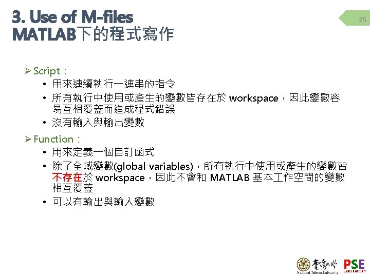
4. Flow-Control Statements for loop Loop Command 1. for 迴圈 Example: • 語法 1： for 變數=向量 運算式 end • 語法 2： for 變數=矩陣 運算式 end 47 Functions: 1. frintf(‘ %d’, i) 2. %d: decimal notation 3. t: provides horizontal tab 4. n: next line For further information: https: //www. mathworks. com/help/matlab _prog/formatting-strings. html >>x=1; >> for i=1: 5 >> x=x*i; >> end >> disp(x) >> x=[1 3; 2 4]; >> for i=x >> fprintf(‘Now I = %dtn', i) >> end Result: Now i = 1 Now i = 2 Now i = 3 Now i = 4 PSE LABORATORY

4. Flow-Control Statements while loop Loop Command 2. while 迴圈 • 語法： while 條件式 運算式 end 48 Example: Is 1+ ε < 1? e= 1; while (1+e) > 1 %判斷式成立 e = e/2; end e = e*2 PSE LABORATORY

4. Flow-Control Statements if branch 49 Branching Command 1. if 條件指令 • 語法： if 條件式一 運算式一 elseif 條件式二 運算式二 elseif 條件式三 運算式三 else 運算式四 end Example: if x > 10 y = log(x) elseif x >= 0 y = sqrt(x) else y = exp(x) - 1 end PSE LABORATORY

4. Flow-Control Statements switch branch Example: Branching Command 2. switch 條件指令 • 語法： switch 運算式 case 值一 運算式一 case 值二 運算式二 otherwise 運算式三 end 50 for month=1: 12 switch month case {3, 4, 5} season='Spring'; case {6, 7, 8} season='Summer'; case {9, 10, 11} season='Autumn'; otherwise season='Winter'; end fprintf('Month %d is %s. n', month, season) % %d for numbers, %s for strings end Result: Month 1 is Winter. Month 2 is Winter. Month 3 is Spring. …. . Month 12 is Winter. PSE LABORATORY

4. Flow-Control Statements Termination of execution 51 Øend: Terminate execution of flow control statement Øbreak: Terminate execution of for or while loop Øreturn: Return to invoking function Example: for i = 1: 1000 if prod(1: i) > 1 e 10 break; % %跳出迴圈 end disp(i) det. m %DET det(A) is the determinant of A. function d = det(A) if isempty(A) d = 1; return else. . . end PSE LABORATORY

Exercise 52 ANSWER myfun. m function C=myfun(B) while B > 2 B=B-1; end C=B^2; clear clc clear all A=[1 2 3 4]'; B(1)=A(1); C(1)=A(1); for i=2: length(A) if A(i)>=3 B(1, i)=A(i)+C(i-1); else B(1, i)=A(i)+B(i-1); end C(1, i)=myfun(B(i)); end Matrix. BC =B*C' PSE LABORATORY

5. Plotting and Graphing 1. 2. 3. 4. 5. 6. 7. 8. 53 Plotting Commands Function – plot Data Markers, Line Types, and Colors Title and Axes Multiple plots on a single figure Plot Tools 3 D Line plot Mesh plot (3 D) PSE LABORATORY

5. Plotting and Graphing Basic Plotting Commands 54 Command Description axis([xmin xmax ymin ymax]) Sets the minimum and maximum limits of x- and y-axes. fplot(’string’, [xmin xmax]) fplot (’string’, [xmin xmax ymin ymax]) Performs intelligent plotting of functions, where ’string’ is a text string that describes the function to be plotted and [xmin xmax] specifies the minimum and maximum values of the independent variable. grid Displays gridlines at the tick marks corresponding to the tick labels. Type grid on to add gridlines; type grid off to stop plotting gridlines. When used by itself, grid switched this feature on or off. plot(x, y) Generates a plot of the array x on rectilinear axes. legend('leg 1', 'leg 2', . . . ) Creates a legend using the strings leg 1, leg 2, and so on and specifies its placement with the mouse. print Prints the plot in the figure window. title('text') Puts text in a title at the top of a plot. xlabel('text') Adds a text label to the x-axis(the abscissa). ylabel('text') Adds a text label to the y-axis(the ordinate). hold Freezes the current plot for subsequent graphics commands. subplot(m, n, p) Splits the figure window into an array of subwindows with m rows and n columns and directs the subsequent plotting commands to the pth subwindow. text(x, y, 'text') Places the string text in the figure window at point specified by coordinates x, y. PSE LABORATORY

5. Plotting and Graphing Function – plot 55 Øplot: 繪圖指令的根本 plot(X, Y, format)：將vector Y 對vector X 做圖 Example: >> clear; clc >> close all >> X=[0: 0. 1: 2*pi]; >> Y=sin(X); >> plot(X, Y, 'bx-') plot(x-data, y-data, ‘color marker line-type') PSE LABORATORY

5. Plotting and Graphing Data Markers, Line Types, and Colors Data markers Line types Dot (．) . Solid line - Black * Dashed line -- Blue x Dash-dotted line -. Cyan Asterisk (*) Cross (×) Circle (。) o Dotted line Colors : k b c Green g + Magenta s Red d White p Yellow Plus sign (+) Square (□) Diamond (◇) Five-point star (★) 56 m r w y Tips: Command Line: help plot PSE LABORATORY

5. Plotting and Graphing Title and Axes 57 Example: close all X=[0: 0. 1: 2*pi]; Y=sin(X); plot(X, Y, 'b--', 'linewidth', 3) title('Y vs X', 'fontsize', 15) xlabel('X', 'fontsize', 15) ylabel('f(X)', 'fontsize', 15) legend('sin(X)') set(gca, 'fontsize', 15) PSE LABORATORY

5. Plotting and Graphing Multiple plots on a single figure 2 59 Øplot(X 1, Y 1, format 1, X 2, Y 2, format 2. . . ) 將 Yi 對 Xi 以 formati 做圖 Example: >> close all; >> X=[0: 0. 1: 2*pi]; >> Y=sin(X); >> Z=cos(X); >> plot(X, Y, 'bx-', X, Z, 'r: ') PSE LABORATORY

5. Plotting and Graphing Multiple plots on a single figure 3 60 Ø使用 hold on重疊多個數對圖形： Example: >> close all; >> X=[0: 0. 1: 2*pi]; >> Y=sin(X); >> Z=cos(X); >> plot(X, Y, 'b--') >> hold on; >> xlabel('X') >> ylabel('f(X)') >> plot(X, Z, 'r: ') >> text(0. 2, 0, 'sin(X)') >> text(0. 5*pi+0. 2, 0, 'cos(X)') PSE LABORATORY

5. Plotting and Graphing Multiple plots on a single figure 4 61 Ø使用 subplot 分割視窗呈現數個子圖形： Example: >> close all; >> X=[0: 0. 1: 2*pi]; >> Y=sin(X); >> Z=cos(X); >> subplot(211); >> plot(X, Y, 'b--') >> xlabel('X') >> ylabel('sin(X)') >> subplot(2, 1, 2); >> plot(X, Z, 'r: ') >> xlabel('X') >> ylabel('cos(X)') PSE LABORATORY

5. Plotting and Graphing Plot Tools 62 Ø Change your graph manually Show plot tool Hide plot tool PSE LABORATORY

5. Plotting and Graphing Plot Tools 63 Generate Code PSE LABORATORY

5. Plotting and Graphing 三維基本繪圖簡介 – line plot 64 Example: close all t = 0: pi/50: 10*pi; plot 3(sin(t), cos(t), t, 'b') title('bf 3 D Curve', 'fontsize', 20) xlabel('sin(t)', 'fontsize', 16) ylabel('cos(t)', 'fontsize', 8) zlabel('it Time') grid on axis square PSE LABORATORY

5. Plotting and Graphing 三維基本繪圖簡介 – mesh plot 65 Example: close all % Generate X and Y arrays for 3 D plots [X, Y] = meshgrid(-3: . 125: 3); Z = peaks(X, Y); % mesh, meshc, meshz Mesh plots mesh(X, Y, Z); axis([-3 3 -10 10]) colorbar PSE LABORATORY

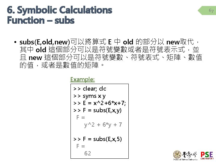
6. Symbolic Calculations 1. 2. 3. 4. 5. 6. 66 Function – subs Function – solve Function – limit Function – diff, int Laplace transform Characteristic Equations and Roots PSE LABORATORY

6. Symbolic Calculations Function – solve 68 Ø 有三種使用solve函數的方式。 Examples: 要求解方程式 x + 5 = 0 >> clear >> clc >> eq 1 = 'x+5=0'; >> solve(eq 1) ans = -5 >> clear >> clc >> solve('x+5=0') ans = -5 >> clear >> clc >> syms x >> solve(x+5) ans = -5 PSE LABORATORY

6. Symbolic Calculations Function – limit 69 Example: 函數 limit(E) 可以用來求出 當 x → 0的時候 E 的極限。 Example: 另外limit(E, v, a)這個形式可以用來 求出當u → a 時的極限。 >> clear; clc >> syms a x >> limit(sin(a*x)/x) ans = a >> clear; clc >> syms h x >> limit((x-3)/(x^2 -9), 3) ans = 1/6 >> limit((sin(x+h)-sin(x))/h, h, 0) ans = cos(x) PSE LABORATORY

6. Symbolic Calculations Function – diff, int syms x f=sin(x); c=diff(f) d=diff(f, 2) c_value=subs(c, 2) d_value=subs(d, 2) c= cos(x) d= -sin(x) c_value = -0. 4161 d_value = -0. 9093 70 syms x y f=sin(x)+cos(y); c=diff(f, x) c 2=diff(f, x, 2) d=diff(f, y) d 2=diff(f, y, 2) syms x f=-2*x/(1+x^2)^2; c=int(f) d=int(f, 0, 1) c= cos(x) c 2 = -sin(x) d= -sin(y) d 2 = -cos(y) c= 1/(1+x^2) d= -1/2 PSE LABORATORY

6. Symbolic Calculations Laplace transform 71 Example: Laplace transform Example: Inverse of Laplace transform >> clear; clc >> syms b t >> laplace(t^3) ans = 6/s^4 >> laplace(exp(-b*t)) ans = 1/(s+b) >> laplace(sin(b*t)) ans = b/(s^2+b^2) >> clear; clc; >> syms b s >> ilaplace(1/s^4) ans = t^3/6 >> ilaplace(1/(s+b)) ans = exp(-b*t) >> ilaplace(b/(s^2+b^2)) ans = sin(b*t) PSE LABORATORY

6. Symbolic Calculations Characteristic Equations and Roots 72 Example: >>clear; clc >> syms k >> A = [0 , 1; -k, -2]; >> charpoly(A) ans = [ 1, 2, k] >> solve(ans) ans = Empty sym: 0 -by-1 >> solve(ans(3)) ans = 0 % old versions of MATLAB have poly(A) >> poly(A) ans = x^2+2*x+k >> solve(ans) ans = [ -1+(1 -k)^(1/2) ] [ -1 -(1 -k)^(1/2) ] PSE LABORATORY

7. Curve Fitting – Regression 73 1. Polynomial Regression Function 2. Curve Fitting Tools PSE LABORATORY

7. Curve Fitting – Regression Functions for Polynomial Regression 74 Command Description p = polyfit(x, y, n) Fits a polynomial of degree n to data described by the vectors x and y, where x is the independent variable. Returns a row vector p of length n + 1 that contains the polynomial coefficients in order of descending powers. [p, s, mu] = polyfit(x, y, n) Fits a polynomial of degree n to data described by the vectors x and y, where x is the independent variable. Returns a row vector p of length n + 1 that contains the polynomial coefficients in order of descending powers and a structure s for use with polyval to obtain error estimates for predictions. The optional output variable mu is two-element vector containing the mean and standard deviation of x. Example: >> p = polyfit(x, y, 1) p= 5 -1 % The linear function y = mx + b with m = 5, b = -1. PSE LABORATORY

7. Curve Fitting – Regression Curve Fitting Tools ① 1. 2. 3. 4. 75 Create a data set in editor or in command window. APP => Curve fitting Transfer data to curve fitting tool Choose a fitting model PSE LABORATORY

7. Curve Fitting – Regression Curve Fitting Tools ② 76 1. Change name 2. Choose x, y data 3. Choose fitting method (Ex. 2 nd order polynomial, auto fit) 4. File => Print to Figure PSE LABORATORY

8. Summary & Supplemental Materials 77 1. Summary of coding 2. Example problems 3. Supplemental materials PSE LABORATORY

8. Summary & Supplemental Materials Summary of coding 1. 2. 3. 4. 5. 78 Write down your logic before coding Look for help in MATLAB Use recognizable names of variables Check matrix dimensions Check loops and iterations PSE LABORATORY

79 Example Problems PSE LABORATORY

80 Examples 1. Convert 2 AD(16) to binary, octal, and decimal system. 2. Convert 11011011011(2) to decimal and hexadecimal system. 3. Find Reynolds number when ρ = 997 kg/m 3, D = 0. 9 m, υ = 4. 8 m/s and μ =0. 89 (kg/m-s). Is it laminar or turbulent flow? (Hint: Re = ρυD/μ) 4. The force required to compress a linear spring is given by the equation F=kx, where F is the force [N], k is the spring constant i [N/m] and x is the compressed distance [m]. The potential energy stored in the compressed spring is given by the equation E=1/2 kx 2, where E is the energy in [J]. Determine compressed distance of each spring and the potential energy stored in each spring. Which spring has the most energy stored in? Spring 1 Spring 2 Spring 3 Spring 4 Force (N) 200 300 250 180 Spring constant k (N/m) 2000 2900 3200 4500 PSE LABORATORY

81 Examples 5. Determine the height of the triangle. Two angles are known as = 30° and = 60°. ? cm =35 o =68 o 80 cm 6. Determine the value of conjugate of (A+B), absolute number of A*B, and remainder after division of real part of A and real part of B, where A=7+3 i, B=2 -i. 7. Create your own matrices A and B with dimensional of 3 x 3 (each value must be in between 0~10), and find the values as follows. a) A. *B b) A*B c) A. /B d) A/B e) 3*A+B^2 8. Find B, C, B+C, B dot C, B cross C when matrices A, B, C are given as: ü A=[2 9 6 3; 3 8 -2 7; 0 1 2 3] ü B=A/2 ü C=A+3 PSE LABORATORY

82 Examples 9. When density = 1000, viscosity = 1, d=0. 5 -4. 0 (interval=0. 5), u =1 -8 (interval =1). Construct a table to represent the diameter (d) to velocity (u) as follows. Re = 500 1000 1500 2000 2500 3000 3500 4000 1000 2000 3000 4000 5000 6000 7000 8000 1500 3000 4500 6000 7500 9000 10500 12000 2500 3000 3500 4000 5000 6000 7000 8000 6000 7500 9000 10500 12000 8000 10000 12000 14000 16000 10000 12500 15000 17500 20000 12000 15000 18000 21000 24000 17500 21000 24500 28000 16000 20000 24000 28000 32000 Table = 1. 0 e+04 * 0 0. 0001 0. 0002 0. 0003 0. 0004 0. 0001 0. 0500 0. 1000 0. 1500 0. 2000 0. 2500 0. 3000 0. 3500 0. 4000 0. 0002 0. 1000 0. 2000 0. 3000 0. 4000 0. 5000 0. 6000 0. 7000 0. 8000 0. 0003 0. 1500 0. 3000 0. 4500 0. 6000 0. 7500 0. 9000 1. 0500 1. 2000 0. 0004 0. 2000 0. 4000 0. 6000 0. 8000 1. 0000 1. 2000 1. 4000 1. 6000 0. 0005 0. 2500 0. 5000 0. 7500 1. 0000 1. 2500 1. 5000 1. 7500 2. 0000 0. 0006 0. 3000 0. 6000 0. 9000 1. 2000 1. 5000 1. 8000 2. 1000 2. 4000 0. 0007 0. 3500 0. 7000 1. 0500 1. 4000 1. 7500 2. 1000 2. 4500 2. 8000 0. 0008 0. 4000 0. 8000 1. 2000 1. 6000 2. 0000 2. 4000 2. 8000 3. 2000 PSE LABORATORY

83 Examples 10. Create your own matrix (dimension of 5*5). Find B, C, and D as in the diagram on the right. 11. Create your own matrix (dimension of 5 x 5) (each value must be in between -5 -5). Find its max value. 12. Determine the maximum, minimum, average, summation, product, standard deviation, determinant, rank, inverse matrix, eigenvalues when the date is given as follows. Data = [120, -80, 181, 132; 5, 19, 22, 34; 3, 8, 1, 9; 177, 65, 9, 17] 13. Write a program that can input three coefficients m, n, p on the command window and calculate the roots of the equation mx 2+nx+p=0. Also output the answer using “disp” and “fprintf” on the command window. Hints: 1. use “input” function: x = input(‘x = ? n’) 2. disp(X) displays the array. If X is a string, the text is displayed. 3. fprintf(FID, FORMAT, A, . . . ) applies the FORMAT to all elements of array A and writes the data to a text file. A = 1 9 10 9 9 1 8 7 1 9 6 2 9 2 1 1 7 5 2 4 9 6 5 4 6 B = 8 7 2 9 7 5 C = 5 D = 8 7 9 rotate B 2 7 5 PSE LABORATORY

84 Examples 14. Create a 10 x 10 random matrix called “mat_10” (all values in between 0 -10). Find the position of the elements equal to zero and output using fprintf. 15. Use “subplot” function and plot the following six equations on one figure (= 6 graphs on one figure and curves should not overlap) Given range: -2π<=t<=2 π 1. sin(t) 2. cos(t) 3. sin(t-pi/2) 4. cos(t-pi/2) 5. sin(t)*cos(t) 6. sin(t 2)*cos(t 2) 14. Output as below mat_10 = 7 1 4 3 7 3 9 8 4 5 7 8 6 6 3 5 7 9 7 0 7 4 4 1 8 3 2 3 4 5 6 4 4 5 7 10 7 4 8 1 1 9 9 3 10 4 1 10 1 9 6 8 2 6 4 6 7 7 3 10 8 5 7 4 3 6 4 6 3 5 0 5 6 8 5 4 5 3 8 5 6 8 1 4 9 2 2 7 1 5 9 5 6 4 6 1 2 4 7 7 z= 20 46 Z= 20 46 �生 0的位置 = 20 �生 0的位置 = 46 Position of 0 = 20 Position of 0 = 46 PSE LABORATORY

Examples 85 16. Plot y= sin(x), y 2=cos(x), and y 3=sin(x)*cos(x) in the range of 0 -2 pi. The line style of y is real black line, y 2 is dotted yellow line, and y 3 is dashed blue line. Add three texts (y=sin(x), y=cos(x), y=sin(x)*cos(x)) beside each curve so that it’s clear each curve is from which equation. • Title: Example 16 (boldface, fontsize = 16). • X-label: x (boldface, fontsize=14) • Y-label: y (boldface, fontsize=14) 17. Plot the surface and contour of the following equations: 1. z = x 2 + 2 xy + y 2 2. z = xy 3. z = x 2 -2 xy - y 2 4. z = x 2 + y 2 Ranges: -5 x 5 and -5 y 5 Hint: You can use “subplot” or “figure” to draw your graphs. PSE LABORATORY

86 Examples 18. Plot a function y=i(x-2)2+5 x+3 where i=-11, -10, -9… 14, 15 and -5<x<5. • For even numbers of i: blue line • For odd numbers of i: red line 19. Use switch case (+ otherwise) and write a programming code to convert NTD/USD/EURO/JPY. If users input a wrong code, print “Wrong Input” so that they know they mistyped. Currency Converter provides the following data (16 th August 2019) • 1 USD = 31. 35*NTD • 1 EURO = 34. 74*NTD • 1 JPY = 0. 30*NTD 20. Van der Waals equations is written as: P=RT/(V-b)-a/V 2 where R=0. 08206, a =8. 664, b=0. 08446. Determine the gas pressure (P) while temperature (T) and volume (V) are entered on the command window (Hint: Use “input” function). Write a program named VDW and a function named PVT to calculate the pressure and transfer the variables R, a, b via “global”. PSE LABORATORY

87 Answers to Examples 1. Convert 2 AD(16) to binary, octal, and decimal system. 1010101101(2), 1255(8), 685(10) 2. Convert 11011011011(2) to decimal and hexadecimal system 1755(10), 6 DB(16) 3. >> clear; clc >> density = 997; D = 0. 9; >> u = 4. 8; >> viscosity = 0. 89; >> Re = density*D*u/viscosity Re = 4839. 4 => turbulent flow 5. Let h be the height of the triangle >> h = 80 / [tan(68*pi/180) tan(35*pi/180)] H is 45. 07 cm. 4. >> clc; clear >> F=[200 300 250 180]; >> k = [2000 2900 3200 4500]; >> x= F. /k x= 0. 1000 0. 1034 0. 0781 0. 0400 >> E=0. 5*k. *x. ^2 E= 10. 0000 15. 5172 9. 7656 3. 6000 Spring 2 has the highest Potential Energy PSE LABORATORY

88 Answers to Examples 6. clc; clear A=7+3 i; B=2 -i; conj(A+B) % conjugate of (A+B) = 9 -2 i abs(A*B) % absolute (A*B) = 17. 0294 rem(real(A), real(B)) % remainder = 1 7. clc; clear A=ceil(10*rand(3, 3)); % your matrix B=magic(3); % your matrix ans 1=A. *B ans 2=A*B ans 3=A. /B ans 4=A/B ans 5=3*A+B^2 8. B= 1. 0000 4. 5000 3. 0000 1. 5000 4. 0000 -1. 0000 3. 5000 0 0. 5000 1. 0000 1. 5000 C= 5 12 9 6 6 11 1 10 3 4 5 6 >> B+C ans = 6. 0000 16. 5000 12. 0000 7. 5000 15. 0000 0 13. 5000 3. 0000 4. 5000 6. 0000 7. 5000 >> dot(B, C) ans = 14 100 31 53 >> cross(B, C) ans = 4. 5000 10. 5000 -6. 0000 -3. 0000 -12. 0000 -6. 0000 0 -1. 5000 12. 0000 -6. 0000 PSE LABORATORY

89 Answers to Examples 9. clc clear density = 1000; viscosity=1; d= 0. 5: 4; u=1: 8; Re= u'*density*d /viscosity Table=[0, d; u', Re] 11. clc; clear A = round(10*rand(5, 5))-5 Max_value=max(A)) 12. 1. max(Data) = 177 65 181 132 2. min(Data)= 3 -80 9 3. mean(Data) = 76. 2500 3. 0000 53. 2500 48. 0000 4. sum(Data) = 305 12 213 192 5. prod(Data) = 318600 10. clc clear A=ceil(10*rand(5, 5)) B=A(2: 4, 2: 3) C=A(15) D=reshape(B, 2, 3) 1 -790400 35838 686664 6. std(Data) = 86. 6155 60. 5915 85. 6052 56. 9620 7. det(Data) = 3. 8958 e+06 8. rank(Data) = 4 9. inv(Data) = [0. 0023 -0. 0224 0. 0436 0. 0040; -0. 0073 0. 0646 -0. 1473 0. 0056; -0. 0037 0. 0869 -0. 2829 0. 0049; 0. 0062 -0. 0596 0. 2590 -0. 0069] 10. eig(Data) = [231. 8609; -108. 5922; 37. 8223; -4. 0910] PSE LABORATORY

Answers to Examples 90 13. clc clear m = input('m=? n'); n = input('n=? n'); p = input('p=? n'); t = n*n-4*m*p; x = [(-n+sqrt(t))/(2*m), (-n-sqrt(t))/(2*m)]; disp(['disp’s results: ', 'x 1= ', num 2 str(x(1)), ' x 2= ', num 2 str(x(2))]) fprintf('fprintf x 1= %7. 4 g + %7. 4 g i, x 2= %7. 4 g + %7. 4 g in', real(x(1)), imag(x(1)), real(x(2)), imag(x(2))) 14. clc; clear mat_10 = round(10*rand(10, 10)) z=find(mat_10 ==0) Z=reshape(z, 1, length(z)) fprintf('產生 0的位置 = %gn', Z) fprintf('Position of 0 = %gn', Z) PSE LABORATORY

Answers to Examples 15. clear; clc close all t=linspace(-2*pi, 100); subplot(3, 2, 1) plot(sin(t)) title('bfsin(t)') subplot(3, 2, 2) plot(cos(t)) title('bfcos(t)') subplot(3, 2, 3) plot(sin(t-pi/2)) title('bfsin(t-pi/2)') subplot(3, 2, 4) plot(cos(t-pi/2)) title('bfcos(t-pi/2)') subplot(3, 2, 5) plot(sin(t). *cos(t)) title('bfsin(t)*cos(t)') subplot(3, 2, 6) plot(sin(t. ^2). *cos(t. ^2)) title('bfsin(t^{2})*cos(t^{2})') 91 PSE LABORATORY

Answers to Examples 92 16. clear; clc; close all x=linspace(0, 2*pi, 1000); plot(x, sin(x), '-k', x, cos(x), '. y', x, sin(x). *cos(x), '--b') title('bf{Example 16}', 'fontsize', 16) xlabel('bf{X}', 'fontsize', 14) ylabel('bf{Y}', 'fontsize', 14) gtext('sin(x)') gtext('cos(x)') gtext('sin(x)*cos(x)') PSE LABORATORY

93 Answers to Examples 17. subplot clear; clc; close all x = -5: 0. 5: 5; y = x; [X, Y] = meshgrid(x, y); subplot(2, 2, 1); surfc(X, Y, X. ^2+2*X. *Y+Y. ^2) subplot(2, 2, 2); surfc(X, Y, X. *Y) subplot(2, 2, 3); surfc(X, Y, X. ^2 -2*X. *Y-Y. ^2) subplot(2, 2, 4); surfc(X, Y, X. ^2+Y. ^2) colormap hot shading interp 17. figure clear; clc; close all x = -5: 0. 5: 5; y = x; [X, Y] = meshgrid(x, y); surfc(X, Y, X. ^2+2*X. *Y+Y. ^2) figure; surfc(X, Y, X. *Y) figure; surfc(X, Y, X. ^2 -2*X. *YY. ^2) figure; surfc(X, Y, X. ^2+Y. ^2) colormap hot shading interp PSE LABORATORY

Answers to Examples 94 18. clear clc close all for i = -11: 2: 15 x = -5: 5; y = i*(x-2). ^2+5*x+3; plot(x, y, 'r') hold on end for i = -10: 2: 14 x = -5: 5; y = i*(x-2). ^2+5*x+3; plot(x, y, 'b') end set(gca, 'xtick', -5: 5) PSE LABORATORY

Answers to Examples 95 19. clear clc % Note: 1 USD = 31. 35*NTD, 1 EURO = 34. 74*NTD, 1 JPY = 0. 30*NTD format bank A = input('input the valuen'); B = input('input the unit (NTD, USD, EURO, JPY)n', 's'); switch B case {'NTD'} x = A/31. 35; % NTD to USD y = A/34. 74; % NTD to EURO z = A/0. 30; % NTD to JPY fprintf('%g USD = %g EURO = %g JPY = %g NTDn', x, y, z, A) case {'EURO'} x = A*34. 74; % EURO to NTD y = x/31. 35; % NTD to USD z = x/0. 3; % NTD to JPY fprintf('%g USD = %g EURO = %g JPY = %g NTDn', y, A, z, x) case {'USD'} x = A*31. 35; % USD to NTD y = x/34. 74; %NTD to EURO z = x/0. 3; % NTD to JPY fprintf('%g USD = %g EURO = %g JPY = %g NTDn', A, y, z, x) case {'JPY'} x = A*0. 3; % JPY to NTD y = x/34. 74; % NTD to EURO z = x/31. 35; % NTD to USD fprintf('%g USD = %g EURO = %g JPY = %g NTDn', z, y, A, x) otherwise fprintf('Wrong Input') end PSE LABORATORY

Answers to Examples 96 20. function VDW_eq clear; clc; global R a b R=0. 08206; a=8. 664; b=0. 08446; T=input('Input the temperature (T) = n'); V=input('Input the volume (V) = n'); P=PVT(T, V) fprintf('n T=%. 2 f K, V=%. 2 f L, P=%. 2 f atmn', T, V, P) function P=PVT(T, V) global R a b P=R*T/(V-b) + a/V^2; PSE LABORATORY

Thank You for Your Attention PSE LABORATORY

98 Supplemental Materials 1. 2. 3. 4. 5. 6. 7. 8. 9. 10. 11. 12. Numerical Differentiation Numerical Integration Interpolation Minimization (optimization) *Solving Algebraic Equation (e. g. fsolve) *Simulink Solving ODE using dee Debug Solving ODE using S-function Simulating LTI model Simulate LTI model using Simulink Solving PDE *important PSE LABORATORY

99 1. Numerical Differentiation True Slope PSE LABORATORY

1. Numerical Differentiation (diff) 100 d = diff(x) = [x(2) − x(1), x(3) − x(2), . . . , x(n) − x(n − 1)] Example: x=0: 0. 1: 1; y=[0. 5 0. 6 0. 7 0. 9 1. 2 1. 4 1. 7 2. 0 2. 4 2. 9 3. 5]; dx=diff(x); dy=diff(y); dydx=diff(y). /diff(x) dydx = 1. 0000 2. 0000 3. 0000 4. 0000 5. 0000 6. 0000 PSE LABORATORY

1. Numerical Differentiation Functions Command Description b = polyder(p) Returns a vector b containing the coefficients of the derivative of the polynomial represented by the vector p. b=polyder(p 2, p 1) Returns a vector b containing the coefficients of the derivative of the polynomial that is the product of the polynomials represented by p 2 and p 1. 101 [n, d]=polyder(p 2, p 1) Returns the vectors n and d containing the coefficients of the numerator and denominator polynomials of the derivative of the quotient p 2/p 1, where p 2 and p 1 are polynomials. PSE LABORATORY

1. Numerical Differentiation (Polynomial Derivatives) 102 p 1 = [5, 2]; p 2 = [10, 4, -3]; der 2 = polyder(p 2) prod = polyder(p 2, p 1) [num, den] = polyder(p 2, p 1) der 2 = 20 4 prod = 150 80 -7 num = 50 40 23 den = 25 20 4 PSE LABORATORY

103 2. Numerical Integration PSE LABORATORY

2. Numerical Integration Command Description trapz(x, y) Uses trapezoidal integration to compute the integral of y with respect to x, where the array y contains the function values at the points contained in the array x quad(’function’, a, b, tol) Uses an adaptive Simpson’s rule to compute the integral of the function ’function’ with a as the lower integration limit and b as the upper limit. The parameter tol is optional. tol indicates the specified error tolerance. 104 quad 1(’function’, a, b, tol Uses Lobatto quadrature to compute the integral of ) the function ’function’. The rest of the syntax is identical to quad. PSE LABORATORY

2. Numerical Integration 105 Examples: x = linspace(0, pi, 10); y = sin(x); trapz(x, y) ans = 1. 9797 x = linspace(0, pi, 100); y = sin(x); trapz(x, y) ans = 1. 9998 x = linspace(0, pi, 1000); y = sin(x); trapz(x, y) ans = 2. 0000 PSE LABORATORY

106 3. Interpolation PSE LABORATORY

3. Interpolation Polynomial Interpolation Functions (1 D) 107 y_est=interp 1(x, y, x_est, 'method') This command specifies alternate methods. The default is linear interpolation. Available methods are: nearest - nearest neighbor interpolation linear - linear interpolation spline - piecewise cubic spline interpolation (SPLINE) pchip - piecewise cubic Hermite interpolation (PCHIP) cubic - same as ’pchip’ PSE LABORATORY

3. Interpolation Polynomial Interpolation Functions (2 D) 108 z_est=interp 2(x, y, z, x_est, y_est, ’method’) This command specifies alternate methods. The default is linear interpolation. Available methods are: nearest - nearest neighbor interpolation linear - bilinear interpolation (or bilinear) spline - cubic spline interpolation (SPLINE) cubic - bicubic interpolation PSE LABORATORY

109 4. Minimization (optimization) PSE LABORATORY

4. Minimization Minimizing a Function of Variables (fminsearch) minimum of 110 , near (0, 0) function f = f 146(x) f = x(1). *exp(-x(1). ^2 -x(2). ^2); %% end, stored in f 145. m fminsearch(@f 146, [0, 0]) % [f, fval] = fminsearch(’f 146’, [0, 0]) ans = -0. 7071 0. 0000 PSE LABORATORY

4. Minimization Other Built-in Functions 111 • fmincon: find minimum of constrained nonlinear multivariable function • fminbnd: find minimum of single-variable function on fixed interva • Isqlin: constrained linear least-squares problems Equation • lsqnonlin: Solve nonlinear least-squares (nonlinear datafitting) problems • quadprog: Solve quadratic programming problems PSE LABORATORY

4. Minimization Optimization Tool 112 PSE LABORATORY

113 5. Solving Algebraic Equation PSE LABORATORY

5. Solving Algebraic Equation Finding Roots of Equations Equation Type Polynomial roots continuous function of one variable nonlinear equations 114 solver roots fzero fsolve (fminsearch…) PSE LABORATORY

5. Solving Algebraic Equation 115 roots Øroots: polynomial roots • syntax： x = roots([c 1 c 2 c 3…. cn+1]) Example: p = [1 -6 -72 -27] r = roots(p) r= 12. 1229 -5. 7345 -0. 3884 PSE LABORATORY

5. Solving Algebraic Equation Some Polynomial Functions Command Description poly(r) Computes the coefficients of the polynomial whose roots are specified by the array r. The resulting coefficients are arranged in descending order of powers. polyval(a, x) Evaluates a polynomial at specified values of its independent variable x. The polynomial’s coefficients of descending powers are stored in the array a. The result is the same size as x. roots(a) Computes an array containing the roots of a polynomial specified by the coefficient array a. 116 PSE LABORATORY

5. Solving Algebraic Equation Polynomial Roots x 3 - 7 x 2 + 40 x -34 =0 roots = 1, 3 ± 5 i a = [1, -7, 40, -34], . . . roots(a) r = [1, 3+5 i, 3 -5 i], . . . poly(r) a= 1 -7 40 -34 r= 1. 00 3. 00+5. 00 i 3. 00 -5. 00 i ans = 3. 000 + 5. 000 i 3. 000 - 5. 000 i 1. 000 117 ans = 1 -7 40 -34 PSE LABORATORY

5. Solving Algebraic Equation fzero 函數 118 Ø fzero: find root of continuous function of one variable • syntax： x = fzero(@FUN, x 0) x：解 FUN：定義問題的 function M-file 檔名 x 0：初始猜值矩陣 PSE LABORATORY

5. Solving Algebraic Equation Example - fzero func 01. m 119 function f=func 01(x) f = sin(x) - cos(x); >> fzero('func 01', [0 3]) ans = 0. 7854 >> fzero('func 01', [3 6]) ans = 3. 9270 PSE LABORATORY

5. Solving Algebraic Equation fsolve 函數 120 Øfsolve: 解聯立方程式 • 語法： x = fsolve(@FUN, x 0) x：解 FUN：定義問題的 function M-file 檔名 x 0：初始猜值矩陣 • Reamark：fsolve() 是 optimization toolbox 的指令 PSE LABORATORY

5. Solving Algebraic Equation Example - fsolve 121 Example: Method 1 Method 2 function F=func 01(X) A=[1 7 5; 2 3 4; 9 6 8]; b=[ 2 ; 4; 6]; F=A*X-b x 0=[1 1 1] x=fsolve('func 01', x 0) x= -0. 4000 -1. 1077 2. 0308 % Use help fsolve for details A=[1 7 5; 2 3 4; 9 6 8]; b=[ 2 ; 4; 6]; c=inv(A)*b x= -0. 4000 -1. 1077 2. 0308 PSE LABORATORY

5. Solving Algebraic Equation Example 122 Ø Van de Vusse (VDV) reaction in an isothermal CSTR: PSE LABORATORY

5. Solving Algebraic Equation Example vdv_sol_ad. m x 0=[2; 1. 117]; k 1=5/6; k 2=5/3; k 3=1/6; fov=4/7; caf=10; options=optimset('Display', 'it er'); [x]=fsolve(@vdv_ae, x 0, option s, k 1, k 2, k 3, fov, caf); cas=x(1) cbs=x(2) 123 vdv_ad. m function F = vdv_ae(x, k 1, k 2, k 3, fov, caf) F = [fov*(caf-x(1))-k 1*x(1)-k 3*(x(1)^2); -fov*x(2)+k 1*x(1)-k 2*x(2)]; PSE LABORATORY

124 6. Simulink PSE LABORATORY

6. SIMULINK Simulink 簡介 125 Ø什麼是 Simulink ? p MATLAB 提供的一個 toolbox p 應用於動態系統模擬 p 提供 GUI，使動態系統的建立如同畫方塊圖(Block Diagram) PSE LABORATORY

6. SIMULINK 啟動 Simulink 126 • 啟動 Simulink： • 直接在 command window 鍵入 「simulink」 • 使用 具列的 Simulink 按鈕： PSE LABORATORY

6. SIMULINK 啟動 Simulink 127 • Simulink 的外觀： PSE LABORATORY

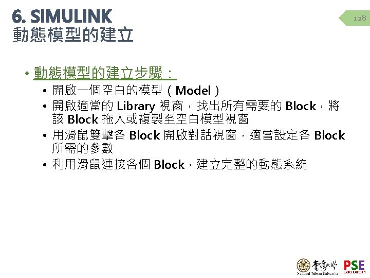
6. SIMULINK 動態模型的建立 129 Open a blank Simulink file Add blocks and connect them PSE LABORATORY

130 7. Solving ODE using dee PSE LABORATORY

7. Solving ODE using dee 啟動指令 131 啟動 dee： • 直接在 command window 鍵入「dee」 A simulnk window named dee will appear PSE LABORATORY

7. Solving ODE using dee 模型建立 132 Connect blocks and add equations PSE LABORATORY

7. Solving ODE using dee 執行指令與作圖 133 k 1=5/6; k 2=5/3; k 3=1/6; fov=4/7; caf=10; x 0=[2; 1. 117]; sim('vdv_sim_4', [0 5]) subplot(2, 1, 1) plot(t, ca) xlabel('t') ylabel('ca') subplot(2, 1, 2) plot(t, cb) xlabel('t') ylabel('cb') PSE LABORATORY

134 8. Debug PSE LABORATORY

8. Debug mode 135 breakpoint Run vdv_sol_ae. m PSE LABORATORY

8. Debug mode (cont’d) 136 Step Continue PSE LABORATORY

137 9. Solving ODE using S-function PSE LABORATORY

9. Solving ODE using S-function Example – VDV reaction 138 Enter search term Constant S-function PSE LABORATORY

Command Line: 139 open sfuntmpl. m will appear PSE LABORATORY

9. Solving ODE using S-function vdv_sfun. m 140 function [sys, x 0, str, ts] = vdv_sfun(t, x, u, flag, x 0) switch flag, case 0, [sys, x 0, str, ts]=mdl. Initialize. Sizes(x 0); case 1, sys=mdl. Derivatives(t, x, u); case 2, sys=mdl. Update(t, x, u); case 3, sys=mdl. Outputs(t, x, u); case 4, sys=mdl. Get. Time. Of. Next. Var. Hit(t, x, u); case 9, sys=mdl. Terminate(t, x, u); otherwise DAStudio. error('Simulink: blocks: unhandled. Flag', num 2 str(flag)); end PSE LABORATORY

9. Solving ODE using S-function vdv_sfun. m (cont’d) 141 function [sys, x 0, str, ts]=mdl. Initialize. Sizes(x 0) sizes = simsizes; sizes. Num. Cont. States = 2; sizes. Num. Disc. States = 0; sizes. Num. Outputs sizes. Num. Inputs = 2; sizes. Dir. Feedthrough = 0; sizes. Num. Sample. Times = 1; % at least one sample time is needed sys = simsizes(sizes); str = []; ts = [0 0]; PSE LABORATORY

9. Solving ODE using S-function vdv_sfun. m (cont’d) function sys=mdl. Derivatives(t, x, u) function sys=mdl. Outputs(t, x, u) ca=x(1); sys = [x(1); x(2)]; 142 cb=x(2); fov=u(1); caf=u(2); k 1=5/6; k 2=5/3; k 3=1/6; dcadt=fov*(caf-ca)-k 1*ca-k 3*(ca^2); function sys=mdl. Get. Time. Of. Next. Var. Hit(t, x, u) sys = []; function sys=mdl. Terminate(t, x, u) sys = []; dcbdt=-fov*cb+k 1*ca-k 2*cb; sys = [dcadt; dcbdt]; function sys=mdl. Update(t, x, u) sys = []; PSE LABORATORY

9. Solving ODE using S-function Example – VDV reaction (cont’d) 143 1 2 4 3 PSE LABORATORY

9. Solving ODE using S-function Example – VDV reaction (cont’d) 144 Command Line: x 0=[2; 1. 117] PSE LABORATORY

9. Solving ODE using S-function Example – VDV reaction (cont’d) 145 sfun_plot. m subplot(2, 1, 1) plot(t, ca) xlabel('t') ylabel('ca') subplot(2, 1, 2) plot(t, cb) xlabel('t') ylabel('cb') PSE LABORATORY

9. Solving ODE using S-function MV step change 146 Step PSE LABORATORY

Command Line: 147 x 0=[3; 1. 117] Start Simulation Reach the new Steady State PSE LABORATORY

9. Solving ODE using S-function Refine Simulink file 148 PSE LABORATORY

9. Solving ODE using S-function Refine Simulink file (cont’d) 149 Create Subsystem in mouse right click menu PSE LABORATORY

9. Solving ODE using S-function Refine Simulink file (cont’d) 150 Mask Subsystem in mouse right click menu PSE LABORATORY

9. Solving ODE using S-function Refine Simulink file (cont’d) 151 Add PSE LABORATORY

9. Solving ODE using S-function Refine Simulink file (cont’d) 152 Right double click on subsystem will appear the following window: PSE LABORATORY

153 10. Simulating LTI model PSE LABORATORY

10. Simulating LTI model 的建立 A=[-2. 4048 0; 0. 83333 -2. 2381]; B=[7; -1. 117]; C=[0 1]; D=[0]; vdv_ss=ss(A, B, C, D) num=[-1. 117 3. 1472]; den=[1 4. 6429 5. 3821]; vdv_tf=tf(num, den) vdv_zpk=zpk(2. 817, [-2. 238 -2. 405], -1. 117) vdv_tf 1=tf(vdv_ss) vdv_zpk 1=zpk(vdv_tf 1) vdv_tfd=c 2 d(vdv_tf, 1, 'zoh') vdv_tf 2=tf(num, den, 'Inputdelay', 1) 154 [ys, ts]=step(vdv_tf); plot(ts, ys) [yi, ti]=impulse(vdv_tf); plot(ti, yi) pole(vdv_tf) tzero(vdv_tf) PSE LABORATORY

10. Simulating LTI model 進階分析 155 …continued from the previous page kc=1; figure(1) bode(kc*vdv_tf) figure(2) [mag, phase, w]=bode(kc*vdv_tf) subplot(2, 1, 1), loglog(w, squeeze(mag)) subplot(2, 1, 2), semilogx(w, squeeze(phase)) [Gm, Pm, Wg, Wp]=margin(mag, phase, w) nyquist(kc*vdv_tf) PSE LABORATORY

156 11. Simulate LTI model using Simulink PSE LABORATORY

11. Simulate LTI model using Simulink LTI model 的建立 157 Transfer Fcn PSE LABORATORY

11. Simulate LTI model using Simulink Closed-loop simulation 158 PSE LABORATORY

11. Simulate LTI model using Simulink Closed-loop simulation 159 PID Controller PSE LABORATORY

160 Look Under Mask PSE LABORATORY

161 12. Solving PDE PSE LABORATORY

12. Solving PDE Numerical Methods for PDE (pdepe) 162 pdepe solves PDEs of the form with boundary conditions PSE LABORATORY

12. Solving PDE Numerical Methods for PDE (pdepe) function [c, b, s] = eqn 1(x, t, u, Du. Dx) %EQN 1: MATLAB function M-le that %species %a PDE in time and one space %dimension. c = 1; b = Du. Dx; s = 0; 163 function value = initial 1(x) %INITIAL 1: MATLAB function M-le %that species the initial condition %for a PDE in time and one space %dimension. value = 2*x/(1+x^2); function [pl, ql, pr, qr] = bc 1(xl, ul, xr, ur, t) %BC 1: MATLAB function M-le that %species boundary conditions %for a PDE in time and one space %dimension. pl = ul; ql = 0; pr = ur-1; qr = 0; PSE LABORATORY

12. Solving PDE Numerical Methods for PDE (pdepe) 164 %PDE 1: MATLAB script M-le that solves and plots %solutions to the PDE stored in eqn 1. m m = 0; x = linspace(0, 1, 20); t = linspace(0, 2, 10); %Solve the PDE u = pdepe(m, @eqn 1, @initial 1, @bc 1, x, t); %Plot solution surf(x, t, u); title('Surface plot of solution. '); xlabel('Distance x'); ylabel('Time t'); PSE LABORATORY

End of Supplemental Materials PSE LABORATORY