Introduction to Marine Geospatial Ecology Tools For Pacific

Introduction to Marine Geospatial Ecology Tools For Pacific EBM Practitioners Jason Roberts and Eric Treml 27 -Aug-2008

Duke Marine Geospatial Ecology Lab Duke Main Campus Durham, North Carolina Washington, D. C. Jason Roberts Duke Marine Lab Beaufort, North Carolina Caroline Good Connie Kot Elliott Hazen Lab Director: Dr. Patrick N. Halpin Sarasota, Florida Daniel Dunn Staff and Students: Ben Best Andre Boustany Andrew Dimatteo Ben Donnally Ari Friedlaender Ei Fujioka Erin Labrecque Rob Schick University of Queensland Brisbane, Australia Eric Treml

Talk outline Overview of Marine Geospatial Ecology Tools (MGET) Quick tour of MGET via an example user scenario Connectivity tools Questions

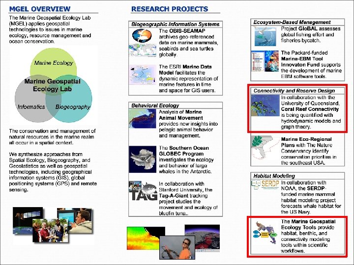
What is MGET? A collection of geoprocessing tools for marine ecology Oceanographic data management and analysis Habitat modeling, connectivity modeling, statistics Highly modular; designed to be used in many scenarios Emphasis on batch processing and interoperability Free, open source Written in Python, R, MATLAB, and C++ Designed mainly for intermediate-skill Arc. GIS users Minimum requirements: Win XP, Arc. GIS 9. 1, Python 2. 4 Arc. GIS and Windows are only non-free requirements

MGET interface in Arc. GIS The MGET toolbox appears in the Arc. Toolbox window

MGET interface in Arc. GIS Drill into the toolbox to find the tools Double-click tools to execute directly, or drag to geoprocessing models to create a workflow

Interoperability MGET “tools” are really just Python functions with input and output parameters: def Do. Something(input 1, input 2, output 1) Python programmers can call MGET functions directly. To facilitate interoperability, MGET exposes these functions as COM Automation objects and Arc. GIS tools. COM-capable program: C / C++ / C#, Visual Basic, R, MATLAB, Java, etc. MGET COM Automation Do. Something class Arc. GIS geoprocessing tool

Example scenario Practitioner has spatially-explicit observations of a species and wants to investigate: Are there spatial and temporal patterns? Correlations with environmental conditions? Correlations with occurrences of other species? Can we predict its occurrence and thereby improve our management of it? By designing MPAs, for example

Typical observation data Fishery catch and bycatch records Surveys IATTC Olive Ridley Encounters 1990 -2005 Argos satellite tracks Figure courtesy of Scott Eckert

Analytic approach 1. Review scientific literature or consult an expert to determine the environmental parameters that might affect the distribution of your species. 2. If possible, measure those parameters when you observe the presence or absence of the species. 3. For parameters you can’t measure at observation time, use software tools to obtain them from remotely-sensed oceanographic data. 4. Build analyze statistical models that try to predict the species’ distribution.

Typical workflow Import species observations into GIS Analyze/model species habitat or behavior MGET includes tools that assist with all of these steps Obtain oceanographic datasets Explore maps of oceano. and observations Sample oceanographic data Prepare oceanographic data for use Create derived oceanographic datasets

Typical workflow Import species observations into GIS Analyze/model species habitat or behavior Obtain oceanographic datasets Explore maps of oceano. and observations Sample oceanographic data Prepare oceanographic data for use Create derived oceanographic datasets

Species observations Skipping the details of this step to save time Ultimately you must produce a point shapefile or feature class that shows locations where the species was present and where it was absent Species presence field: 1 = present, 0 = absent Date field records date of observation

Typical workflow Import species observations into GIS Analyze/model species habitat or behavior Download oceanographic datasets Explore maps of oceano. and observations Sample oceanographic data Prepare oceanographic data for use Create derived oceanographic datasets

Options for obtaining data 1. Download files from data providers using FTP Nearly all data products are available with FTP Powerful, free downloaders exist (e. g. Smart. FTP) But must often convert files to Arc. GIS-compatible formats 2. Download using MGET or other tool (e. g. NOAA EDC) The tool hides details of download, using FTP, OPe. NDAP or other protocols, and writes Arc. GIS-compatible formats Not many such tools exist 3. Order files on CD-ROM or DVD-ROM Use this if your Internet connection is slow

Example MGET tool for downloading data: Download Aviso SSH Dataset to Arc. GIS Rasters

Example SSH and currents data with turtle track

Typical workflow Import species observations into GIS Analyze/model species habitat or behavior Obtain oceanographic datasets Explore maps of oceano. and observations Sample oceanographic data Prepare oceanographic data for use Create derived oceanographic datasets

Preparing oceanography for use Most oceanographic datasets are not immediately usable by Arc. GIS Common preprocessing steps include: Converting to an Arc. GIS-supported format Projecting to a desired projection Clipping to region of interest Performing basic calculations (via map algebra) E. g. converting integers given by the original data provider to floats that represent the real values Building pyramids

A very popular MGET tool: Convert HDF SDS to Arc. GIS Raster

Sea surface temperature NOAA Coast. Watch AVHRR GOES 10/12 from PO. DAAC NOAA NODC 4 km AVHRR Pathfinder v 5 Also: MODIS Aqua and Terra, GOES 9

Sea surface chlorophyll density Sea. Wi. FS from the NASA GSFC Ocean. Color Group Also: MODIS Aqua and combined MODIS/Sea. Wi. FS

Quik. SCAT ocean winds from PO. DAAC 28 -Aug-2005 Katrina Also: BYU Quik. SCAT Sigma-0 (approximates sea surface rougness)

Global bathymetries ETOPO 2 GEBCO S 2004 Map shows S 2004 clipped to eastern Pacific ocean

Typical workflow Import species observations into GIS Analyze/model species habitat or behavior Obtain oceanographic datasets Explore maps of oceano. and observations Sample oceanographic data Prepare oceanographic data for use Create derived oceanographic datasets

AVHRR Daytime SST 03 -Jan 2005 Identifying Surface Temperature Fronts Cayula-Cornillion Edge Detection Algorithm (1992) Mexico Frequency Step 1: Histogram analysis Optimal break 27. 0 °C Bimoda l Temperature 28. 0 °C Step 2: Spatial cohesion test Front 25. 8 °C ~120 km Strong cohesion front present Geoprocessing model Weak cohesion no front Example output Mexico

Typical workflow Import species observation s into GIS Analyze/model species habitat or behavior Obtain oceanograph ic datasets Explore maps of oceano. and observation s Sample oceanograph ic data Prepare oceanograph ic data for use Create derived oceanograph ic datasets

Sampling is the procedure of overlaying points over a map and storing the map’s value as an attribute of each point. Chlorophyll -a Density Chl field filled with values from the map MGET has sampling tools for various scenarios

Typical workflow Import species observation s into GIS Analyze/model species habitat with statistics Obtain oceanograph ic datasets Explore maps of oceano. and observation s Sample oceanograph ic data Prepare oceanograph ic data for use Create derived oceanograph ic datasets

MGET statistics tools Lots of tools, many more planned Built from Ben Best’s Arc. RStats / Hab. Mod projects Tools require the R statistics program to be installed on your computer

Exploratory analysis Density Histogram tool Density Turtle present Turtle absent Distance to nesting beach (m) Scatterplot Matrix tool

Fitting statistical models ROC plots Term plots

Predicting habitat maps from the model Input #3: Rasters for predictor variable s Input #1: The fitted model Predict GAM tool Input #2: Cutoff value Predicted species presence Binary habitat (cutoff = 0. 025) Bayesian probability that predicted presence ≥ 0. 025

Marine Connectivity via Larval dispersal Many marine species • Larval dispersal stage • Sessile or sedentary adults • Space/habitat limited • Ocean currents influence transport • Populations connected via dispersal

Modeling Connectivity Study site Simulating the release of larvae from 450 reefs in the Tropical Pacific - coral reefs

Modeling Connectivity Quantifying arrival probability Modeling larval dispersal via ocean currents using Eulerian advection/diffusion

Modeling Connectivity Graph Structure Summarizing reef-to-reef dispersal using directed graphs

Graph Analysis Example: Potential Sources and Sinks Applying graph theory to better understand connectivity and inform conservation

MGET coral reef connectivity tools Coral reef ID and % cover maps Ocean currents data Tool downloads data for the region and dates you specify Edge list feature class representing dispersal network Larval density time series rasters

Thanks! Download MGET: http: //code. env. duke. edu/projects/mget Jason Roberts jason. roberts@duke. edu Eric Treml e. treml@uq. edu. au