INTRODUCTION TO MANAGEMENT SCIENCE 13 e Anderson Sweeney

INTRODUCTION TO MANAGEMENT SCIENCE, 13 e Anderson Sweeney Williams Martin © 2011 Cengage Learning. All Rights Reserved. May not be scanned, copied or duplicated, or posted to a © 2008 Thomson South-Western. All Rights Reserved publicly accessible website, in whole or in part. Slides by JOHN LOUCKS St. Edward’s University Slide 1

Chapter 3 Linear Programming: Sensitivity Analysis and Interpretation of Solution n n Introduction to Sensitivity Analysis Graphical Sensitivity Analysis: Computer Solution Simultaneous Changes © 2011 Cengage Learning. All Rights Reserved. May not be scanned, copied or duplicated, or posted to a © 2008 Thomson South-Western. All Rights Reserved publicly accessible website, in whole or in part. Slide 2

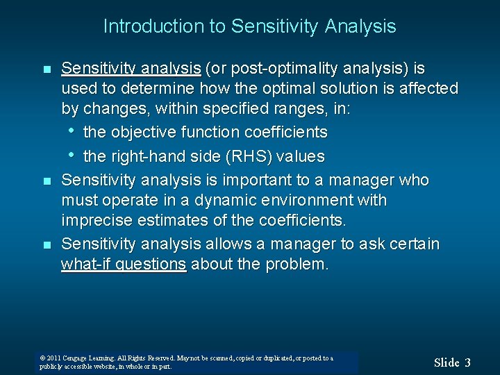
Introduction to Sensitivity Analysis n n n Sensitivity analysis (or post-optimality analysis) is used to determine how the optimal solution is affected by changes, within specified ranges, in: • the objective function coefficients • the right-hand side (RHS) values Sensitivity analysis is important to a manager who must operate in a dynamic environment with imprecise estimates of the coefficients. Sensitivity analysis allows a manager to ask certain what-if questions about the problem. © 2011 Cengage Learning. All Rights Reserved. May not be scanned, copied or duplicated, or posted to a © 2008 Thomson South-Western. All Rights Reserved publicly accessible website, in whole or in part. Slide 3

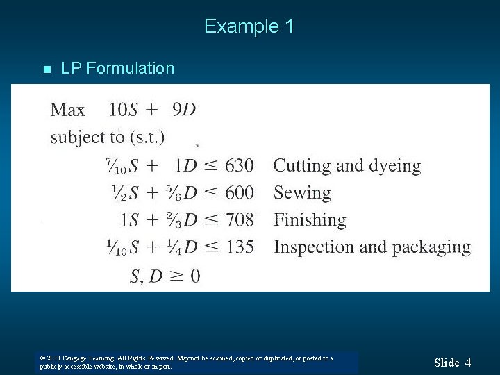
Example 1 n LP Formulation © 2011 Cengage Learning. All Rights Reserved. May not be scanned, copied or duplicated, or posted to a © 2008 Thomson South-Western. All Rights Reserved publicly accessible website, in whole or in part. Slide 4

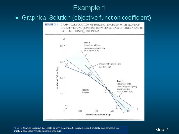
Example 1 n Graphical Solution (objective function coefficient) © 2011 Cengage Learning. All Rights Reserved. May not be scanned, copied or duplicated, or posted to a © 2008 Thomson South-Western. All Rights Reserved publicly accessible website, in whole or in part. Slide 5

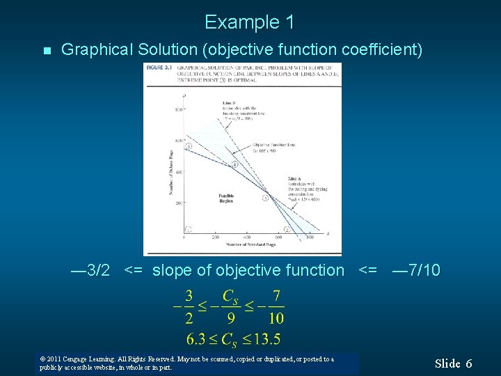
Example 1 n Graphical Solution (objective function coefficient) ― 3/2 <= slope of objective function <= ― 7/10 © 2011 Cengage Learning. All Rights Reserved. May not be scanned, copied or duplicated, or posted to a © 2008 Thomson South-Western. All Rights Reserved publicly accessible website, in whole or in part. Slide 6

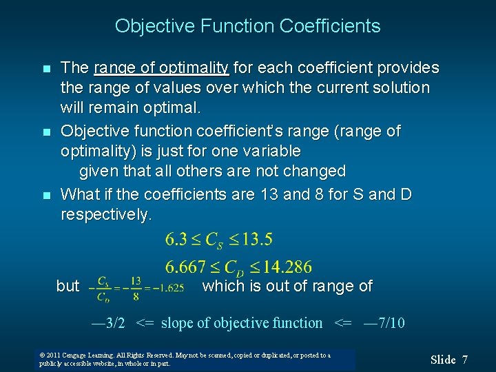
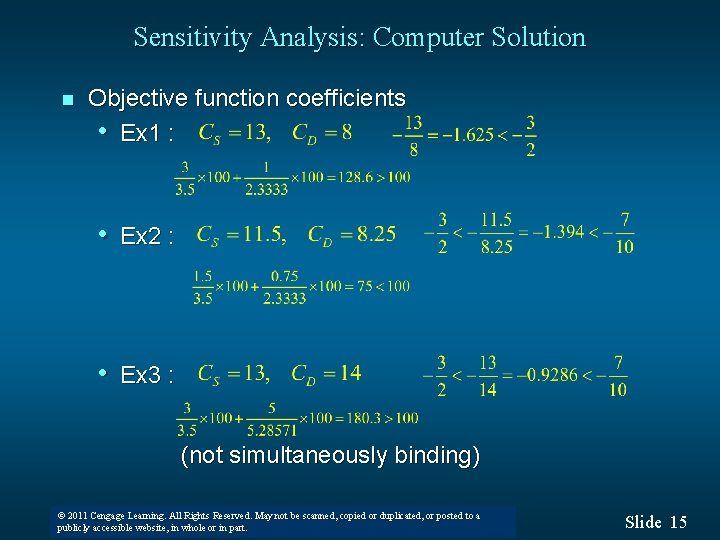
Objective Function Coefficients n n n The range of optimality for each coefficient provides the range of values over which the current solution will remain optimal. Objective function coefficient’s range (range of optimality) is just for one variable given that all others are not changed What if the coefficients are 13 and 8 for S and D respectively. but which is out of range of ― 3/2 <= slope of objective function <= ― 7/10 © 2011 Cengage Learning. All Rights Reserved. May not be scanned, copied or duplicated, or posted to a © 2008 Thomson South-Western. All Rights Reserved publicly accessible website, in whole or in part. Slide 7

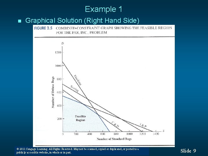
Right-Hand Sides n n Let us consider how a change in the right-hand side for a constraint might affect the feasible region and perhaps cause a change in the optimal solution. The improvement in the value of the optimal solution per unit increase in the right-hand side is called the dual price. The range of feasibility is the range over which the dual price is applicable. As the RHS increases, other constraints will become binding and limit the change in the value of the objective function. © 2011 Cengage Learning. All Rights Reserved. May not be scanned, copied or duplicated, or posted to a © 2008 Thomson South-Western. All Rights Reserved publicly accessible website, in whole or in part. Slide 8

Example 1 n Graphical Solution (Right Hand Side) © 2011 Cengage Learning. All Rights Reserved. May not be scanned, copied or duplicated, or posted to a © 2008 Thomson South-Western. All Rights Reserved publicly accessible website, in whole or in part. Slide 9

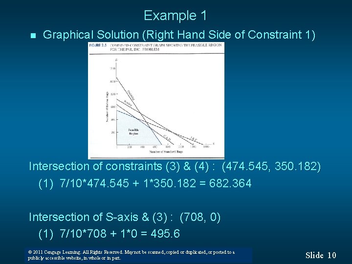
Example 1 n Graphical Solution (Right Hand Side of Constraint 1) Intersection of constraints (3) & (4) : (474. 545, 350. 182) (1) 7/10*474. 545 + 1*350. 182 = 682. 364 Intersection of S-axis & (3) : (708, 0) (1) 7/10*708 + 1*0 = 495. 6 © 2011 Cengage Learning. All Rights Reserved. May not be scanned, copied or duplicated, or posted to a © 2008 Thomson South-Western. All Rights Reserved publicly accessible website, in whole or in part. Slide 10

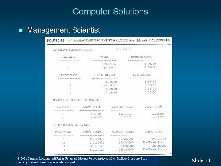
Computer Solutions n Management Scientist © 2011 Cengage Learning. All Rights Reserved. May not be scanned, copied or duplicated, or posted to a © 2008 Thomson South-Western. All Rights Reserved publicly accessible website, in whole or in part. Slide 11

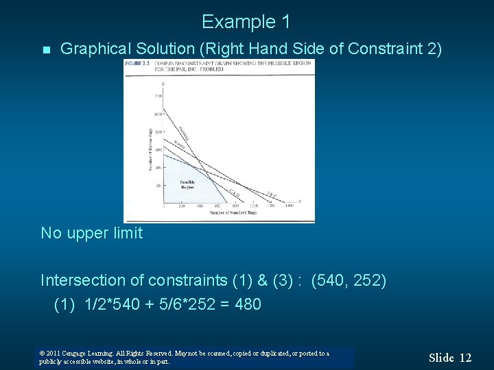
Example 1 n Graphical Solution (Right Hand Side of Constraint 2) No upper limit Intersection of constraints (1) & (3) : (540, 252) (1) 1/2*540 + 5/6*252 = 480 © 2011 Cengage Learning. All Rights Reserved. May not be scanned, copied or duplicated, or posted to a © 2008 Thomson South-Western. All Rights Reserved publicly accessible website, in whole or in part. Slide 12

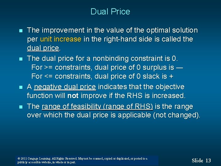
Dual Price n n The improvement in the value of the optimal solution per unit increase in the right-hand side is called the dual price. The dual price for a nonbinding constraint is 0. For >= constraints, dual price of 0 surplus is ― For <= constraints, dual price of 0 slack is + A negative dual price indicates that the objective function will not improve if the RHS is increased. The range of feasibility (range of RHS) is the range over which the dual price is applicable (not changed). © 2011 Cengage Learning. All Rights Reserved. May not be scanned, copied or duplicated, or posted to a © 2008 Thomson South-Western. All Rights Reserved publicly accessible website, in whole or in part. Slide 13

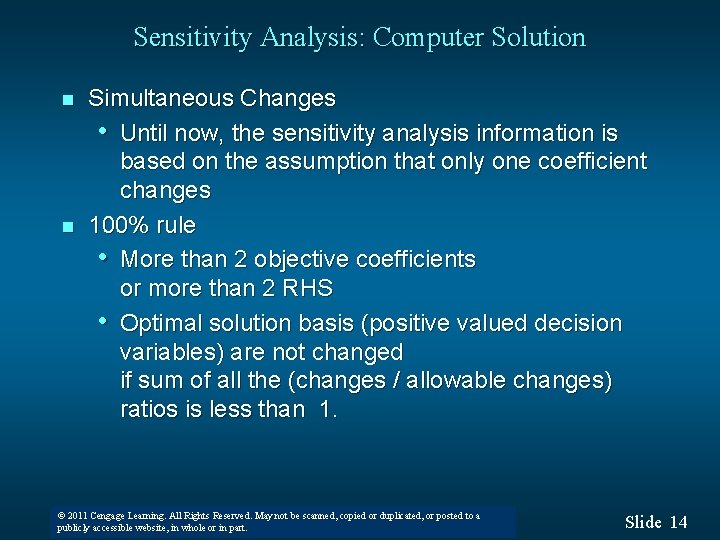
Sensitivity Analysis: Computer Solution n n Simultaneous Changes • Until now, the sensitivity analysis information is based on the assumption that only one coefficient changes 100% rule • More than 2 objective coefficients or more than 2 RHS • Optimal solution basis (positive valued decision variables) are not changed if sum of all the (changes / allowable changes) ratios is less than 1. © 2011 Cengage Learning. All Rights Reserved. May not be scanned, copied or duplicated, or posted to a © 2008 Thomson South-Western. All Rights Reserved publicly accessible website, in whole or in part. Slide 14

Sensitivity Analysis: Computer Solution n Objective function coefficients • Ex 1 : • Ex 2 : • Ex 3 : (not simultaneously binding) © 2011 Cengage Learning. All Rights Reserved. May not be scanned, copied or duplicated, or posted to a © 2008 Thomson South-Western. All Rights Reserved publicly accessible website, in whole or in part. Slide 15

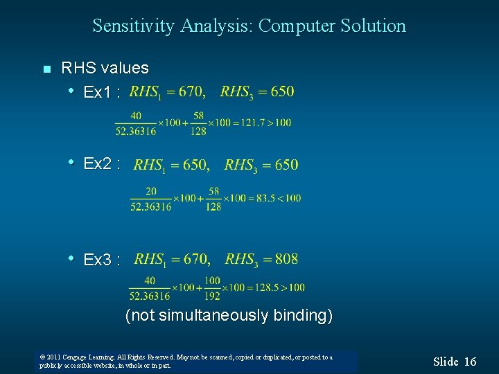
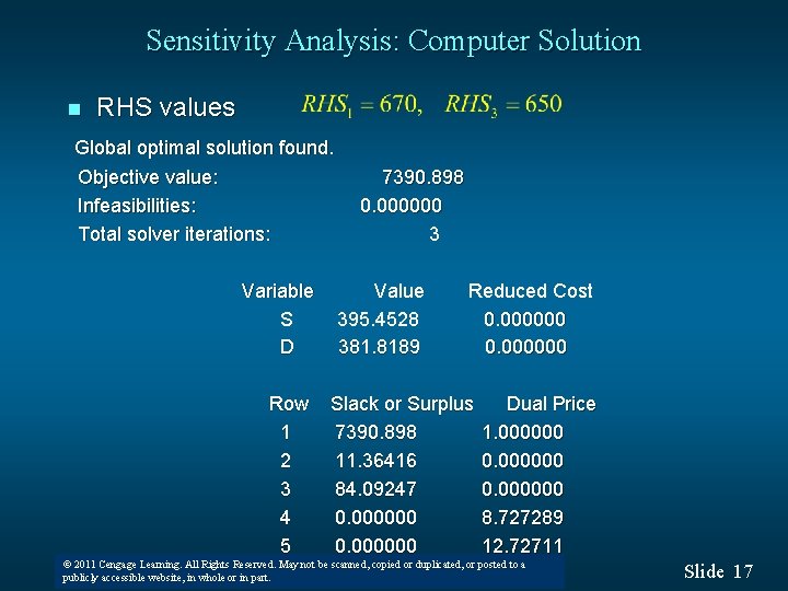
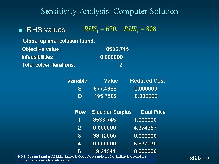
Sensitivity Analysis: Computer Solution n RHS values • Ex 1 : • Ex 2 : • Ex 3 : (not simultaneously binding) © 2011 Cengage Learning. All Rights Reserved. May not be scanned, copied or duplicated, or posted to a © 2008 Thomson South-Western. All Rights Reserved publicly accessible website, in whole or in part. Slide 16

Sensitivity Analysis: Computer Solution n RHS values Global optimal solution found. Objective value: Infeasibilities: Total solver iterations: Variable S D 7390. 898 0. 000000 3 Value 395. 4528 381. 8189 Reduced Cost 0. 000000 Row Slack or Surplus Dual Price 1 7390. 898 1. 000000 2 11. 36416 0. 000000 3 84. 09247 0. 000000 4 0. 000000 8. 727289 5 0. 000000 12. 72711 © 2011 Cengage Learning. All Rights Reserved. May not be scanned, copied or duplicated, or posted to a © 2008 Thomson South-Western. All Rights Reserved publicly accessible website, in whole or in part. Slide 17

Sensitivity Analysis: Computer Solution n RHS values Global optimal solution found. Objective value: 7353. 117 Infeasibilities: 0. 000000 Total solver iterations: 2 Variable S D Value 406. 2477 365. 6266 Reduced Cost 0. 000000 Row Slack or Surplus Dual Price 1 7353. 117 1. 000000 2 0. 000000 4. 374957 3 92. 18853 0. 000000 4 0. 000000 6. 937530 5 2. 968579 0. 000000 © 2011 Cengage Learning. All Rights Reserved. May not be scanned, copied or duplicated, or posted to a © 2008 Thomson South-Western. All Rights Reserved publicly accessible website, in whole or in part. Slide 18

Sensitivity Analysis: Computer Solution n RHS values Global optimal solution found. Objective value: 8536. 745 Infeasibilities: 0. 000000 Total solver iterations: 2 Variable S D Value 677. 4988 195. 7509 Reduced Cost 0. 000000 Row Slack or Surplus Dual Price 1 8536. 745 1. 000000 2 0. 000000 4. 374957 3 98. 12555 0. 000000 4 0. 000000 6. 937530 5 18. 31241 0. 000000 © 2011 Cengage Learning. All Rights Reserved. May not be scanned, copied or duplicated, or posted to a © 2008 Thomson South-Western. All Rights Reserved publicly accessible website, in whole or in part. Slide 19

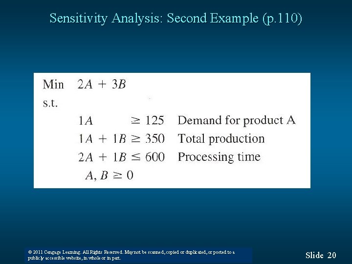
Sensitivity Analysis: Second Example (p. 110) © 2011 Cengage Learning. All Rights Reserved. May not be scanned, copied or duplicated, or posted to a © 2008 Thomson South-Western. All Rights Reserved publicly accessible website, in whole or in part. Slide 20

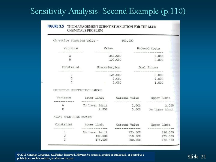
Sensitivity Analysis: Second Example (p. 110) © 2011 Cengage Learning. All Rights Reserved. May not be scanned, copied or duplicated, or posted to a © 2008 Thomson South-Western. All Rights Reserved publicly accessible website, in whole or in part. Slide 21

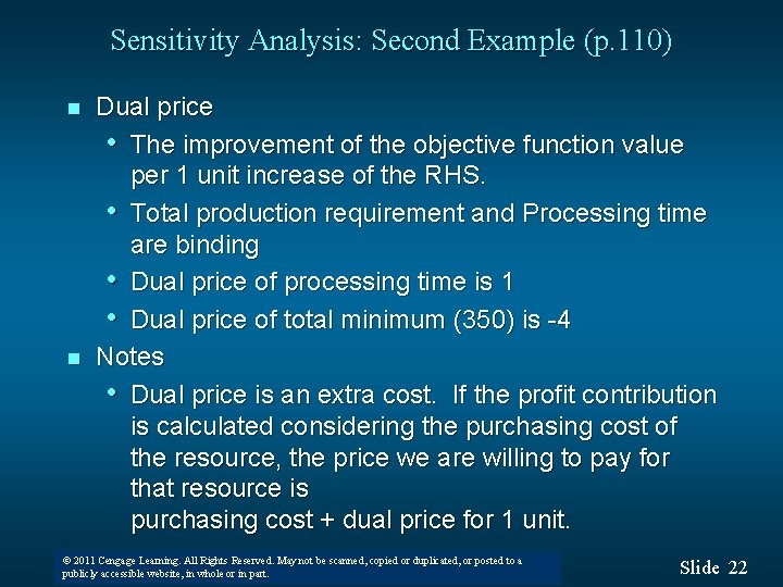
Sensitivity Analysis: Second Example (p. 110) n n Dual price • The improvement of the objective function value per 1 unit increase of the RHS. • Total production requirement and Processing time are binding • Dual price of processing time is 1 • Dual price of total minimum (350) is -4 Notes • Dual price is an extra cost. If the profit contribution is calculated considering the purchasing cost of the resource, the price we are willing to pay for that resource is purchasing cost + dual price for 1 unit. © 2011 Cengage Learning. All Rights Reserved. May not be scanned, copied or duplicated, or posted to a © 2008 Thomson South-Western. All Rights Reserved publicly accessible website, in whole or in part. Slide 22

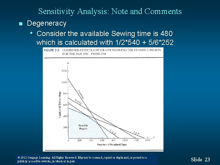
Sensitivity Analysis: Note and Comments n Degeneracy • Consider the available Sewing time is 480 which is calculated with 1/2*540 + 5/6*252 © 2011 Cengage Learning. All Rights Reserved. May not be scanned, copied or duplicated, or posted to a © 2008 Thomson South-Western. All Rights Reserved publicly accessible website, in whole or in part. Slide 23

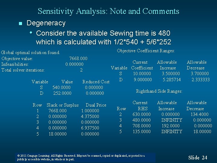
Sensitivity Analysis: Note and Comments n Degeneracy • Consider the available Sewing time is 480 which is calculated with 1/2*540 + 5/6*252 Global optimal solution found. Objective value: Infeasibilities: Total solver iterations: Objective Coefficient Ranges: 7668. 000 0. 000000 2 Variable Value S 540. 0000 D 252. 0000 Row Slack or Surplus 1 7668. 000 2 0. 000000 3 0. 000000 4 0. 000000 5 18. 00000 Current Allowable Variable Coefficient Increase Decrease S 10. 00000 3. 500000 3. 700000 D 9. 000000 5. 285714 2. 333333 Reduced Cost 0. 000000 Righthand Side Ranges: 0. 000000 Dual Price 1. 000000 4. 375000 0. 000000 6. 937500 0. 000000 Row 2 3 4 5 Current RHS 630. 0000 480. 0000 708. 0000 135. 0000 © 2011 Cengage Learning. All Rights Reserved. May not be scanned, copied or duplicated, or posted to a © 2008 Thomson South-Western. All Rights Reserved publicly accessible website, in whole or in part. Allowable Increase Decrease 0. 000000 134. 4000 INFINITY 0. 000000 192. 0000 0. 000000 INFINITY 18. 00000 Slide 24

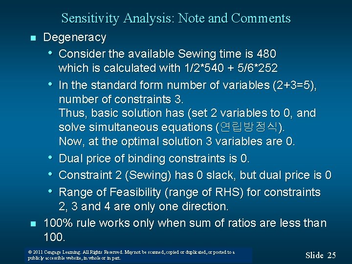
Sensitivity Analysis: Note and Comments n n Degeneracy • Consider the available Sewing time is 480 which is calculated with 1/2*540 + 5/6*252 • In the standard form number of variables (2+3=5), number of constraints 3. Thus, basic solution has (set 2 variables to 0, and solve simultaneous equations (연립방정식). Now, at the optimal solution 3 variables are 0. • Dual price of binding constraints is 0. • Constraint 2 (Sewing) has 0 slack, but dual price is 0 • Range of Feasibility (range of RHS) for constraints 2, 3 and 4 are only one direction. 100% rule works only when sum of ratios are less than 100. © 2011 Cengage Learning. All Rights Reserved. May not be scanned, copied or duplicated, or posted to a © 2008 Thomson South-Western. All Rights Reserved publicly accessible website, in whole or in part. Slide 25

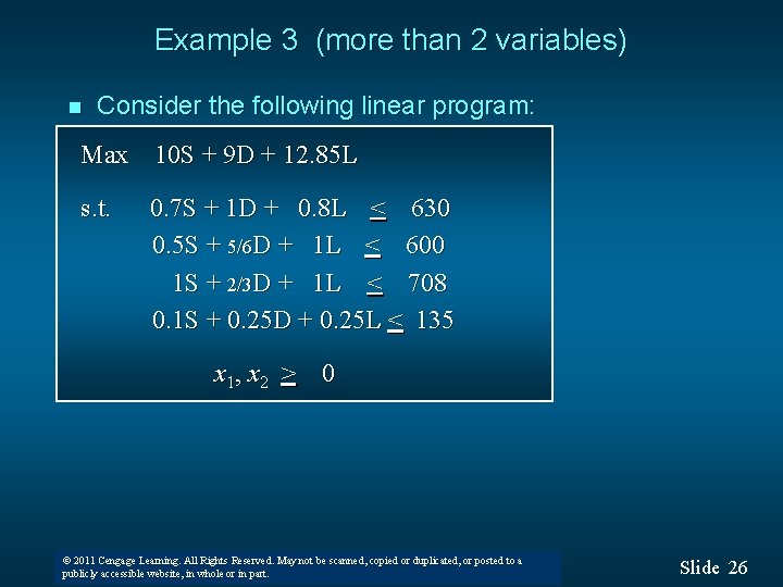
Example 3 (more than 2 variables) n Consider the following linear program: Max 10 S + 9 D + 12. 85 L s. t. 0. 7 S + 1 D + 0. 8 L < 630 0. 5 S + 5/6 D + 1 L < 600 1 S + 2/3 D + 1 L < 708 0. 1 S + 0. 25 D + 0. 25 L < 135 x 1, x 2 > 0 © 2011 Cengage Learning. All Rights Reserved. May not be scanned, copied or duplicated, or posted to a © 2008 Thomson South-Western. All Rights Reserved publicly accessible website, in whole or in part. Slide 26

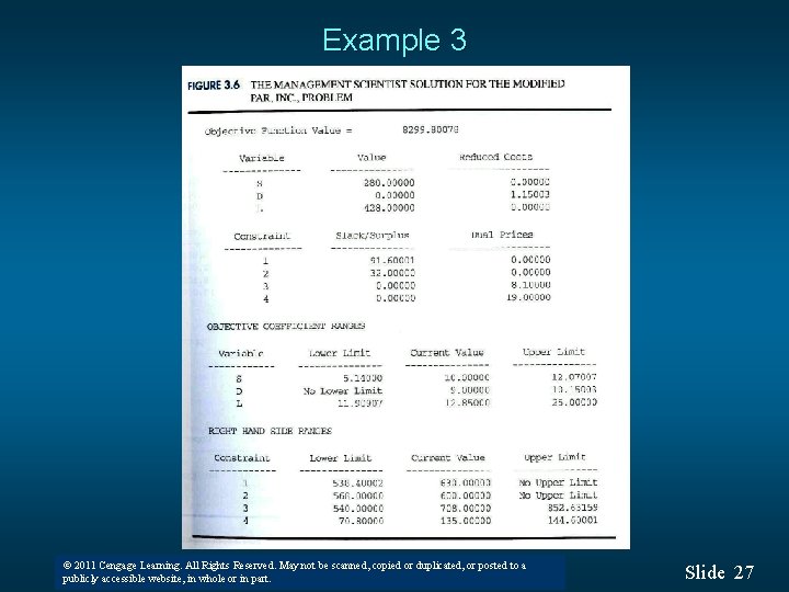
Example 3 © 2011 Cengage Learning. All Rights Reserved. May not be scanned, copied or duplicated, or posted to a © 2008 Thomson South-Western. All Rights Reserved publicly accessible website, in whole or in part. Slide 27

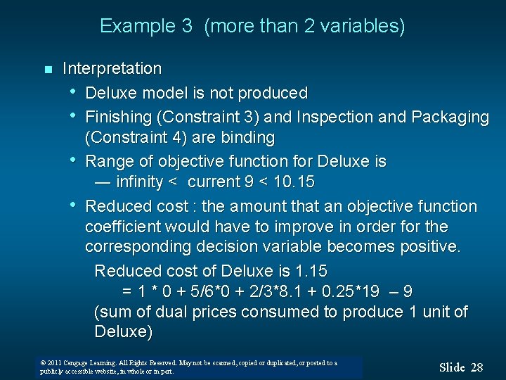
Example 3 (more than 2 variables) n Interpretation • Deluxe model is not produced • Finishing (Constraint 3) and Inspection and Packaging (Constraint 4) are binding • Range of objective function for Deluxe is ― infinity < current 9 < 10. 15 • Reduced cost : the amount that an objective function coefficient would have to improve in order for the corresponding decision variable becomes positive. Reduced cost of Deluxe is 1. 15 = 1 * 0 + 5/6*0 + 2/3*8. 1 + 0. 25*19 – 9 (sum of dual prices consumed to produce 1 unit of Deluxe) © 2011 Cengage Learning. All Rights Reserved. May not be scanned, copied or duplicated, or posted to a © 2008 Thomson South-Western. All Rights Reserved publicly accessible website, in whole or in part. Slide 28

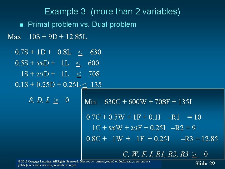
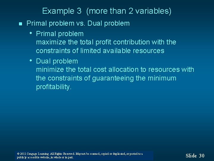
Example 3 (more than 2 variables) n Primal problem vs. Dual problem Max 10 S + 9 D + 12. 85 L 0. 7 S + 1 D + 0. 8 L < 630 0. 5 S + 5/6 D + 1 L < 600 1 S + 2/3 D + 1 L < 708 0. 1 S + 0. 25 D + 0. 25 L < 135 S, D, L > 0 Min 630 C + 600 W + 708 F + 135 I 0. 7 C + 0. 5 W + 1 F + 0. 1 I –R 1 = 10 1 C + 5/6 W + 2/3 F + 0. 25 I –R 2 = 9 0. 8 C + 1 W + 1 F + 0. 25 I –R 3 = 12. 85 C, W, F, I, R 1, R 2, R 3 > 0 © 2011 Cengage Learning. All Rights Reserved. May not be scanned, copied or duplicated, or posted to a © 2008 Thomson South-Western. All Rights Reserved publicly accessible website, in whole or in part. Slide 29

Example 3 (more than 2 variables) n Primal problem vs. Dual problem • Primal problem maximize the total profit contribution with the constraints of limited available resources • Dual problem minimize the total cost allocation to resources with the constraints of guaranteeing the minimum profitability. © 2011 Cengage Learning. All Rights Reserved. May not be scanned, copied or duplicated, or posted to a © 2008 Thomson South-Western. All Rights Reserved publicly accessible website, in whole or in part. Slide 30

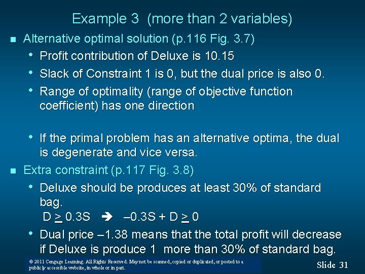
Example 3 (more than 2 variables) n Alternative optimal solution (p. 116 Fig. 3. 7) • Profit contribution of Deluxe is 10. 15 • Slack of Constraint 1 is 0, but the dual price is also 0. • Range of optimality (range of objective function coefficient) has one direction • n If the primal problem has an alternative optima, the dual is degenerate and vice versa. Extra constraint (p. 117 Fig. 3. 8) • Deluxe should be produces at least 30% of standard bag. D > 0. 3 S – 0. 3 S + D > 0 • Dual price – 1. 38 means that the total profit will decrease if Deluxe is produce 1 more than 30% of standard bag. © 2011 Cengage Learning. All Rights Reserved. May not be scanned, copied or duplicated, or posted to a © 2008 Thomson South-Western. All Rights Reserved publicly accessible website, in whole or in part. Slide 31

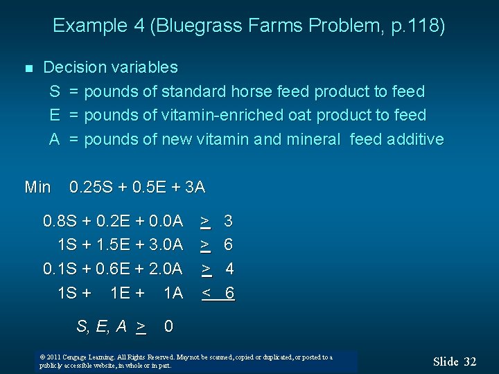
Example 4 (Bluegrass Farms Problem, p. 118) n Decision variables S = pounds of standard horse feed product to feed E = pounds of vitamin-enriched oat product to feed A = pounds of new vitamin and mineral feed additive Min 0. 25 S + 0. 5 E + 3 A 0. 8 S + 0. 2 E + 0. 0 A > 3 1 S + 1. 5 E + 3. 0 A > 6 0. 1 S + 0. 6 E + 2. 0 A > 4 1 S + 1 E + 1 A < 6 S, E, A > 0 © 2011 Cengage Learning. All Rights Reserved. May not be scanned, copied or duplicated, or posted to a © 2008 Thomson South-Western. All Rights Reserved publicly accessible website, in whole or in part. Slide 32

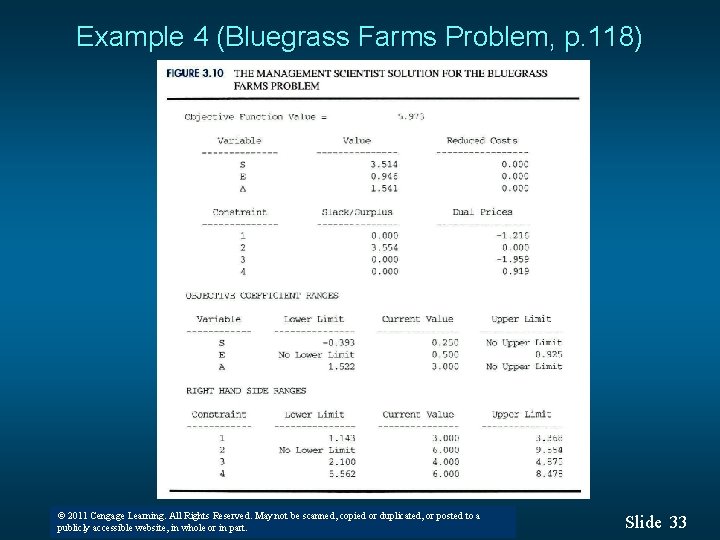
Example 4 (Bluegrass Farms Problem, p. 118) © 2011 Cengage Learning. All Rights Reserved. May not be scanned, copied or duplicated, or posted to a © 2008 Thomson South-Western. All Rights Reserved publicly accessible website, in whole or in part. Slide 33

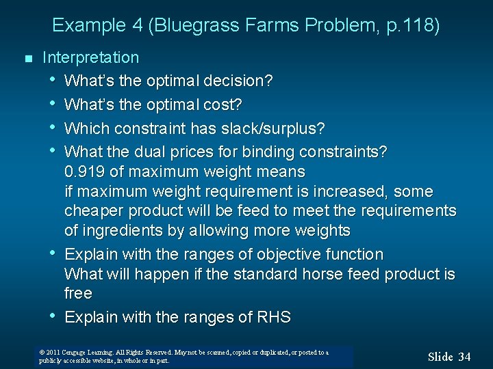
Example 4 (Bluegrass Farms Problem, p. 118) n Interpretation • What’s the optimal decision? • What’s the optimal cost? • Which constraint has slack/surplus? • What the dual prices for binding constraints? 0. 919 of maximum weight means if maximum weight requirement is increased, some cheaper product will be feed to meet the requirements of ingredients by allowing more weights • Explain with the ranges of objective function What will happen if the standard horse feed product is free • Explain with the ranges of RHS © 2011 Cengage Learning. All Rights Reserved. May not be scanned, copied or duplicated, or posted to a © 2008 Thomson South-Western. All Rights Reserved publicly accessible website, in whole or in part. Slide 34

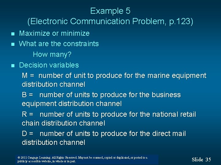
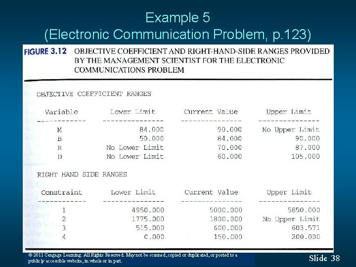
Example 5 (Electronic Communication Problem, p. 123) n n n Maximize or minimize What are the constraints How many? Decision variables M = number of unit to produce for the marine equipment distribution channel B = number of units to produce for the business equipment distribution channel R = number of units to produce for the national retail chain distribution channel D = number of units to produce for the direct mail distribution channel © 2011 Cengage Learning. All Rights Reserved. May not be scanned, copied or duplicated, or posted to a © 2008 Thomson South-Western. All Rights Reserved publicly accessible website, in whole or in part. Slide 35

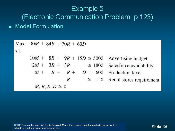
Example 5 (Electronic Communication Problem, p. 123) n Model Formulation © 2011 Cengage Learning. All Rights Reserved. May not be scanned, copied or duplicated, or posted to a © 2008 Thomson South-Western. All Rights Reserved publicly accessible website, in whole or in part. Slide 36

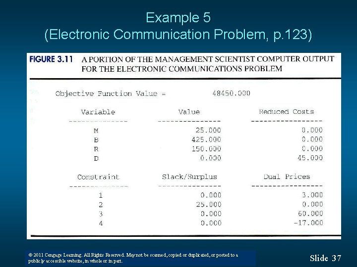
Example 5 (Electronic Communication Problem, p. 123) © 2011 Cengage Learning. All Rights Reserved. May not be scanned, copied or duplicated, or posted to a © 2008 Thomson South-Western. All Rights Reserved publicly accessible website, in whole or in part. Slide 37

Example 5 (Electronic Communication Problem, p. 123) © 2011 Cengage Learning. All Rights Reserved. May not be scanned, copied or duplicated, or posted to a © 2008 Thomson South-Western. All Rights Reserved publicly accessible website, in whole or in part. Slide 38

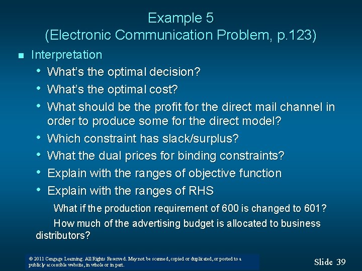
Example 5 (Electronic Communication Problem, p. 123) n Interpretation • What’s the optimal decision? • What’s the optimal cost? • What should be the profit for the direct mail channel in order to produce some for the direct model? • Which constraint has slack/surplus? • What the dual prices for binding constraints? • Explain with the ranges of objective function • Explain with the ranges of RHS What if the production requirement of 600 is changed to 601? How much of the advertising budget is allocated to business distributors? © 2011 Cengage Learning. All Rights Reserved. May not be scanned, copied or duplicated, or posted to a © 2008 Thomson South-Western. All Rights Reserved publicly accessible website, in whole or in part. Slide 39

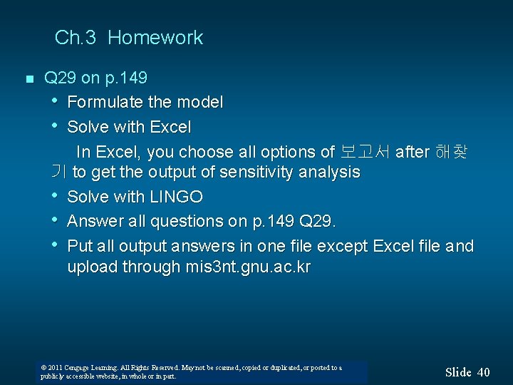
Ch. 3 Homework n Q 29 on p. 149 • Formulate the model • Solve with Excel In Excel, you choose all options of 보고서 after 해찾 기 to get the output of sensitivity analysis • Solve with LINGO • Answer all questions on p. 149 Q 29. • Put all output answers in one file except Excel file and upload through mis 3 nt. gnu. ac. kr © 2011 Cengage Learning. All Rights Reserved. May not be scanned, copied or duplicated, or posted to a © 2008 Thomson South-Western. All Rights Reserved publicly accessible website, in whole or in part. Slide 40

End of Chapter 3 © 2011 Cengage Learning. All Rights Reserved. May not be scanned, copied or duplicated, or posted to a © 2008 Thomson South-Western. All Rights Reserved publicly accessible website, in whole or in part. Slide 41