Introduction to Linear System Theory and simple feedback

Introduction to Linear System Theory and simple feedback PID Controllers EE 125 Ruzena Bajcsy

Linear Systems • Linearity means that the relationship between the input and the output of the system is a linear map: If input • produces response • and input produces response • then the scaled and summed input produces the scaled and summed response where a 1 and a 2 are real scalars.

It follows that it can be extended to any number of terms , c[k]. *Input produces input p produces output Output

Time Invariance • Time invariance means that whether we apply an input to the system now or T seconds from now, the output will be identical except for a time delay of the T seconds. That is, if the output due to input x(t) is y(t), then the output due to input x(t − T) is y(t − T). Hence, the system is time invariant because the output does not depend on the particular time the input is applied.

Fundamental results in Linear System theory • The fundamental result in LTI system theory is that any LTI system can be characterized entirely by a single function called the system's impulse response. The output of the system is simply the convolution of the input to the system with the system's impulse response.

Time domain • This method of analysis is often called the time domain point-of-view. The same result is true of discrete-time linear shift-invariant systems in which signals are discrete-time samples, and convolution is defined on sequences.

• Equivalently, any LTI system can be characterized in the frequency domain by the system's transfer function, which is the Laplace transform of the system's impulse response. As a result of the properties of these transforms, the output of the system in the frequency domain is the product of the transfer function and the transform of the input. In other words, convolution in the time domain is equivalent to multiplication in the

Laplace transform • Laplace transform: definition • Where s is a complex number

The Properties of Laplace Transform • df(t)/dt = s F(s) –f(0) • Integral of f(t) = 1/s F(s) • Show proof of Laplace transform of function derivative

The relationship between Time and frequency domain

Transfer Function • In its simplest form for continuous-time input signal x(t) and output y(t), the transfer function is the linear mapping of the Laplace transform of the input, X(s), to the output Y(s): • Y(s) = H(s). X(s) or

Stability Analysis • A linear time-invariant system without dead time is described completely by the distribution of its poles and zeros and the gain factor. When N(s) =0 we compute the zeros • When D(s) =0 we compute poles.

Poles and zeros

Composition of modules and Feedback • G(s) = Y(s)/U(s) =G[1](s)/(1+- G[1](s). G[2](s))

Pure amplifier examp. • With high gain K infinity • The entire technique of operational amplifier is based on this principle.

Stable (a) and unstable (b) system response

Stability • For stability it is sufficient to check only the • Poles. • 1. Asymptotic stability iff all poles are on the left half plane • 2. Instability is when at least on pole is in the right plane • 3. Critical stability is when at least one pole is on the imaginary axes.

S PLANE

RLC example

State Space representation • Differential equations describing LRC • And initial conditions

State vector • y(t) = u(t)

State differential equations • one obtains the general state-space representation of a linear time-invariant single -input-single-output system: • This is state diff. equation and y(t) is the output equation

State space vs. Transfer function • The key advantage of transfer functions is in their compactness, which makes them suitable for frequency-domain analysis and stability studies. However, the transfer function approach suffers from neglecting the initial conditions. Not only does state-space representation serve as an alternative to transfer functions, but also it is not limited to linear and time-invariant systems and it has the following advantages:

Cont. • The key advantage of transfer functions is in their compactness, • Single-input-single-output and multi-inputmulti-output systems can be formally treated equal. • The state-space representation is best suited both for theoretical treatment of control systems (analytical solutions, optimisation) and for numerical calculations.

Cont. • The determination of the system response in the homogeneous case with the initial condition is very simple. • This representation gives a better insight into the inner system behaviour. General system properties, for example, the system controllability or observability can be defined and determined.

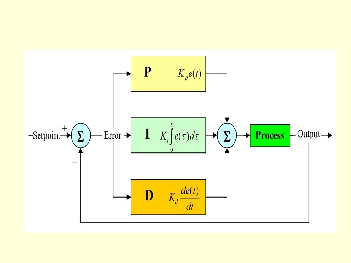
PID controller

The PID CONTROLLER • You've probably seen the terms defined before: P -Proportional, I - Integral, D - Derivative. These terms describe three basic mathematical functions applied to the error signal , Verror = Vset - Vsensor. This error represents the difference between where you want to go (Vset), and where you're actually at (Vsensor).

PID • The controller performs the PID mathematical functions on the error and applies their sum to a process (motor, heater, etc. ) So simple, yet so powerful! If tuned correctly, the signal Vsensor should move closer to Vset. •

THREE MULTIPLIERS • Tuning a system means adjusting three multipliers Kp, Ki and Kd adding in various amounts of these functions to get the system to behave the way you want. The table below summarizes the PID terms and their effect on a control system. •

Term Math Function Proportional KP x Verror Typically the main drive in a control loop, KP reduces a large part of the overall error. Integral KI x ∫ Verror dt Reduces the final error in a system. Summing even a small error over time produces a drive signal large enough to move the system toward a smaller error.

Derivative KD x d. Verror / dt Counteracts the KP and KI terms when the output changes quickly. This helps reduce overshoot and ringing. It has no effect on final error.

Proportional Term(Gain)

Integral term(reset)

Derivative term

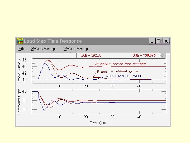
Effects of Proportional feedback • Proportional gain, Kp Larger values typically mean faster response since the larger the error, the larger the proportional term compensation. An excessively large proportional gain will lead to process instability and oscilation.

Effect of Integral feedback • Integral gain, Ki Larger values imply steady state errors are eliminated more quickly. The trade-off is larger overshoot: any negative error integrated during transient response must be integrated away by positive error before reaching steady state.

Effect of derivative feedback • Derivative gain, Kd Larger values decrease overshoot, but slow down transient response and may lead to instability due to signal noise amplification in the differentiation of the error.

How to select the coefficients • TUNING THE PID CONTROLLER • Although you'll find many methods and theories on tuning a PID, here's a straight forward approach to get you up and soloing quickly. • 1. SET KP. Starting with KP=0, KI=0 and KD=0, increase KP until the output starts overshooting and ringing significantly.

Cont. • TUNING THE PID CONTROLLER • 2. SET KD. Increase KD until the overshoot is reduced to an acceptable level. • 3. SET KI. Increase KI until the final error is equal to zero.

Basic Schema • Plant: A System to be Controlled • Controller provides the excitation for the plant

Three Term Controller • The transfer function of the PID Controller • Is here: • Where Kp is proportional gain • KI =integral gain • Kd=differential gain

Error • Set Point (R) is the desired Value • Error is the difference between the output measurement and the set point • Process or Plant

PID controller , schema • Refering to the first slide, The variable (e) represents the tracking error, the difference between the desired input value (R) and the actual output (Y). This error signal (e) will be sent to the PID controller, and the controller computes both the derivative and the integral of this error signal. The signal (u) just past the controller is now equal to the proportional gain (Kp) times the magnitude of the error plus the integral gain (Ki) times the integral of the error plus the derivative gain (Kd) times the derivative of the error.

Intuitive explanation This signal (u) will be sent to the plant, and the new output (Y) will be obtained. This new output (Y) will be sent back to the sensor again to find the new error signal (e). The controller takes this new error signal and computes its derivative and its integral again. This process goes on and on

Example • Simple model for mass, spring and damper

Transfer Function • Taking the Laplace transform of the previous equation • Transfer Function between the displacement and Input

Transfer Function and Stability • Any Laplace domain transfer function can be expressed as the ratio of two polynomials N(s) and D(s) • T(s) =N(s)/D(s) • • – . We define: Zero: the zeros of T(s) are the roots of N(s) = 0, and Pole: the poles of T(s) are the roots of D(s) = 0. Stability of is determined by its poles or simply the roots of the characteristic equation: D(s) = 0. For stability, the real part of every pole must be negative. If T(s) is formed by closing a negative feedback loop around the open-loop transfer function F(s) =A(s)/B(s) , then the roots of the characteristic equation are also the zeros of , or simply the roots of A(s) + B(s).

DC gain • DC gain is a ratio of the steady state. The step response to the magnitude of step function, or where s=0.

Example Transfer function Open loop • • • M = 1 kg b = 10 N. s/m k = 20 N/m F(s) = 1 The DC gain of the plant transfer function is 1/20, so 0. 05 is the final value of the output to an unit step input. This corresponds to the steady-state error of 0. 95, quite large indeed. Furthermore, the rise time is about one second, and the settling time is about 1. 5 seconds. Let's design a controller that will reduce the rise time, reduce the settling time, and eliminates the steady-state error

Proportional Controller • Proportional controller (Kp) reduces the rise time, increases the overshoot, and reduces the steady-state error. The closed-loop transfer function of the above system with a proportional controller is:

PID plot • Open Loop Proportional Loop

Proportional derivative Control • Now, let's take a look at a PD control. From the table shown above, we see that the derivative controller (Kd) reduces both the overshoot and the settling time. The closedloop transfer function of the given system with a PD controller is:

Proportional derivative Control reduced both the overshoot and settling time

Proportional Integral Controler • An integral controller (Ki) decreases the rise time, increases both the overshoot and the settling time, and eliminates the steady-state error. For the given system, the closed-loop transfer function with a PI control is:

Plot for PI controller • We have reduced the proportional gain (Kp) because the integral controller also reduces the rise time and increases the overshoot as the proportional controller does (double effect). The above response shows that the integral controller eliminated the steady-state error

Proportional Integral derivative Controller • After several trial and error runs, the gains Kp=350, Ki=300, and Kd=50 provided the desired response.

THE response of Step input to PID controller • We have obtained performance with no overshoot, fast rise time and no steady state error

Modeling a Cruise Control System

Modeling a Cruise Control System • The model of the cruise control system is relatively simple. If the inertia of the wheels is neglected, and it is assumed that friction (b) (which is proportional to the car's speed) is what is opposing the motion of the car (u is the force from the engine), then the problem is reduced to the simple mass and damper system shown below

Design requirements • m = 1000 kg b = 50 Nsec/m u = 500 N • Design requirements: • The next step in modeling this system is to come up with some design criteria. When the engine gives a 500 Newton force, the car will reach a maximum velocity of 10 m/s (22 mph). An automobile should be able to accelerate up to that speed in less than 5 seconds. Since this is only a cruise control system, a 10% overshoot on the velocity will not do much damage. A 2% steady-state error is also acceptable for the same reason

Design criteria • Keeping the above in mind, we have proposed the following design criteria for this problem: • Rise time < 5 sec Overshoot < 10% Steady state error < 2%

Transfer Function • To find the transfer function of the above system, we need to take the Laplace transform of the modeling equations (1). When finding the transfer function, zero initial conditions must be assumed. Laplace transforms of the two equations are shown below • ms V(s) +b. V(s) =U(s) • Y(s)= V(s)

Transfer Function • We can substitute V(s) in terms Y(s) • ms. Y(s) +b. Y(s) = U(s) • Transfer function is:

State Space Representaion • We can rewrite the first-order modeling equation (1) as the state-space model

Open Loop response • From the plot, we see that the vehicle takes more than 100 seconds to reach the steadystate speed of 10 m/s. This does not satisfy our rise time criterion of less than 5 seconds

Design criteria for the feedback • Rise time < 5 sec Overshoot < 10% Steady state error < 2%

This step meets all the criteria

DC Motor Speed Modeling • A common actuator in control systems is the DC motor. It directly provides rotary motion and, coupled with wheels or drums and cables, can provide transitional motion. The electric circuit of the armature and the free body diagram of the rotor are shown in the following figure:

Physical parameters of this motor • * moment of inertia of the rotor (J) = 0. 01 kg. m^2/s^2 * damping ratio of the mechanical system (b) = 0. 1 Nms * electromotive force constant (K=Ke=Kt) = 0. 01 Nm/Amp * electric resistance (R) = 1 ohm * electric inductance (L) = 0. 5 H * input (V): Source Voltage * output (theta): position of shaft * The rotor and shaft are assumed to be rigid

DC motor modeling • The motor torque, T, is related to the armature current, i, by a constant factor Kt. The back emf, e, is related to the rotational velocity by the following equations:

DC motor modeling • In SI units (which we will use), Kt (armature constant) is equal to Ke (motor constant). • From the figure above we can write the following equations based on Newton's law combined with Kirchhoff's law:

Laplace transfer function • We can get the following open-loop transfer function, where the rotational speed is the output and the voltage is the input

Design criteria • With a 1 rad/sec step input, the design criteria are: • Settling time less than 2 seconds • Overshoot less than 5% • Steady-stage error less than 1%

PID control • Let's try a PID controller with small Ki and Kd. Change your m-file so it looks like the following. Kp=100; Ki=1; Kd=1;

PID control with small Ki and Kd

Tuning the gains • Now the settling time is too long. Let's increase Ki to reduce the settling time. Go back to your m-file and change Ki to 200. Rerun the file and you should get the plot like this:

PID control with large Ki

Further tuning • Now we see that the response is much faster than before, but the large Ki has worsened the transient response (big overshoot). Let's increase Kd to reduce the overshoot. Go back to the m-file and change Kd to 10. Rerun it and you should get this plot:

The right PID control

The final parameters for our motor • So now we know that if we use a PID controller with • Kp=100, Ki=200, Kd=10, • all of our design requirements will be satisfied.