Introduction to Linear Regression and Correlation Analysis Goals

Introduction to Linear Regression and Correlation Analysis

Goals After this, you should be able to: Calculate and interpret the simple correlation between two variables • Determine whether the correlation is significant • Calculate and interpret the simple linear regression equation for a set of data • Understand the assumptions behind regression analysis • Determine whether a regression model is significant •

Goals After this, you should be able to: (continued) • Calculate and interpret confidence intervals for the regression coefficients • Recognize regression analysis applications for purposes of prediction and description • Recognize some potential problems if regression analysis is used incorrectly • Recognize nonlinear relationships between two variables

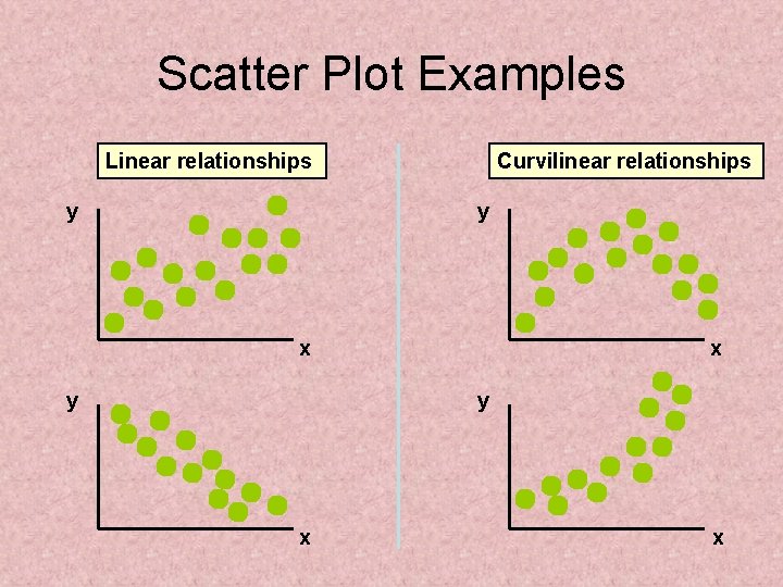
Scatter Plots and Correlation • A scatter plot (or scatter diagram) is used to show the relationship between two variables • Correlation analysis is used to measure strength of the association (linear relationship) between two variables – Only concerned with strength of the relationship – No causal effect is implied

Scatter Plot Examples Linear relationships y Curvilinear relationships y x y x x

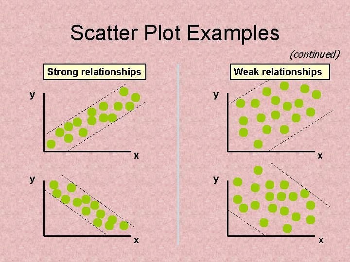
Scatter Plot Examples (continued) Strong relationships y Weak relationships y x y x x

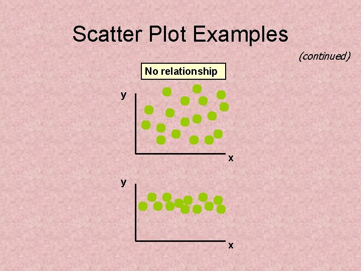
Scatter Plot Examples (continued) No relationship y x

Correlation Coefficient (continued) • The population correlation coefficient ρ (rho) measures the strength of the association between the variables • The sample correlation coefficient r is an estimate of ρ and is used to measure the strength of the linear relationship in the sample observations

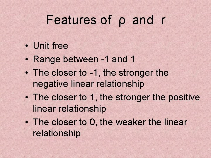
Features of ρ and r • Unit free • Range between -1 and 1 • The closer to -1, the stronger the negative linear relationship • The closer to 1, the stronger the positive linear relationship • The closer to 0, the weaker the linear relationship

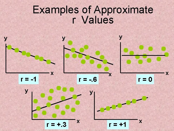
Examples of Approximate r Values y y y r = -1 x r = -. 6 y x r = 0 y r = +. 3 x r = +1 x x

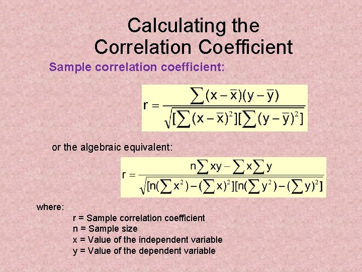
Calculating the Correlation Coefficient Sample correlation coefficient: or the algebraic equivalent: where: r = Sample correlation coefficient n = Sample size x = Value of the independent variable y = Value of the dependent variable

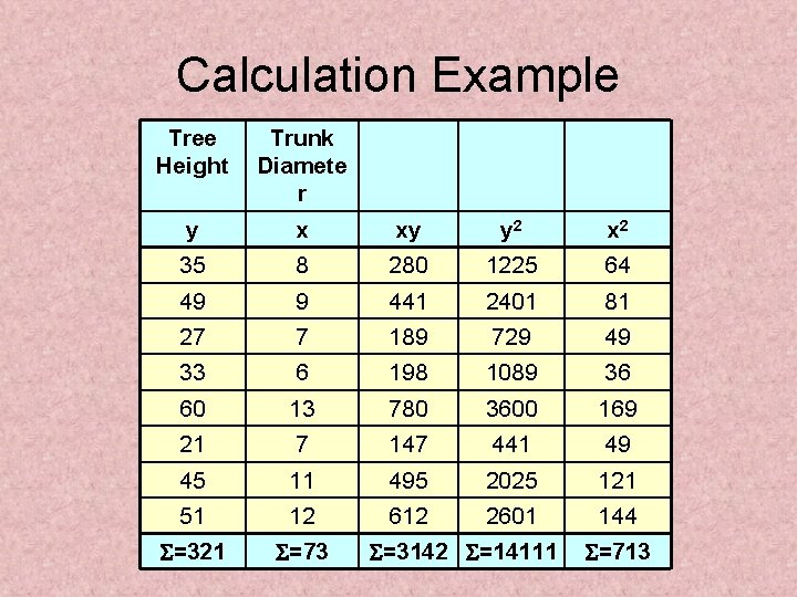
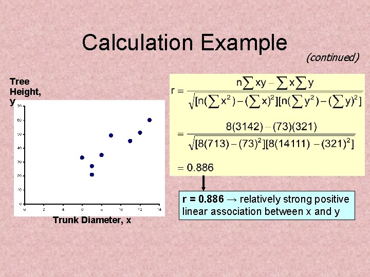
Calculation Example Tree Height Trunk Diamete r y x xy y 2 x 2 35 8 280 1225 64 49 9 441 2401 81 27 7 189 729 49 33 6 198 1089 36 60 13 780 3600 169 21 7 147 441 49 45 11 495 2025 121 51 12 612 2601 144 =321 =73 =3142 =14111 =713

Calculation Example (continued) Tree Height, y Trunk Diameter, x r = 0. 886 → relatively strong positive linear association between x and y

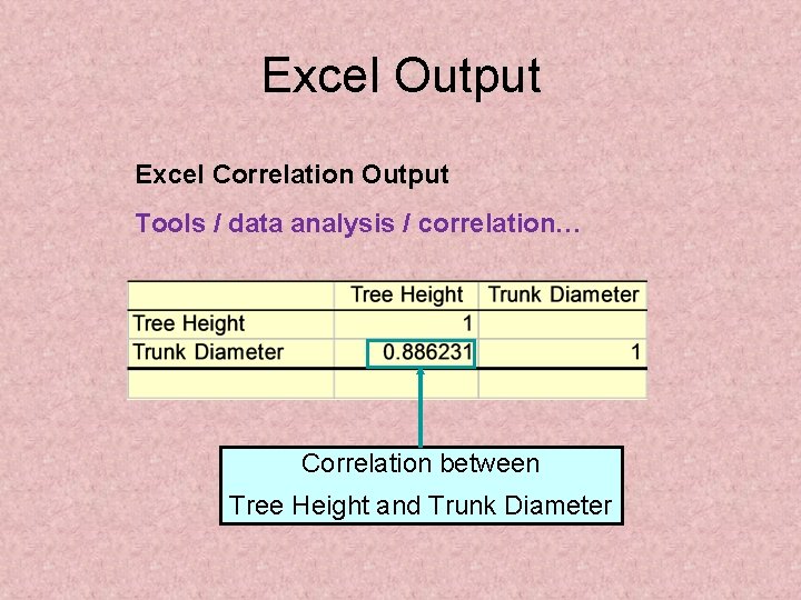
Excel Output Excel Correlation Output Tools / data analysis / correlation… Correlation between Tree Height and Trunk Diameter

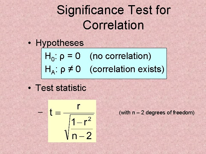
Significance Test for Correlation • Hypotheses H 0: ρ = 0 (no correlation) HA: ρ ≠ 0 (correlation exists) • Test statistic – (with n – 2 degrees of freedom)

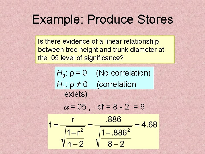
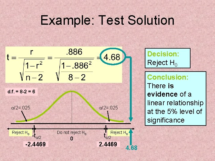
Example: Produce Stores Is there evidence of a linear relationship between tree height and trunk diameter at the. 05 level of significance? H 0: ρ = 0 H 1: ρ ≠ 0 exists) (No correlation) (correlation =. 05 , df = 8 - 2 = 6

Example: Test Solution Decision: Reject H 0 Conclusion: There is evidence of a linear relationship at the 5% level of significance d. f. = 8 -2 = 6 a/2=. 025 Reject H 0 -tα/2 -2. 4469 a/2=. 025 Do not reject H 0 0 Reject H 0 tα/2 2. 4469 4. 68

Introduction to Regression Analysis • Regression analysis is used to: – Predict the value of a dependent variable based on the value of at least one independent variable – Explain the impact of changes in an independent variable on the dependent variable Dependent variable: the variable we wish to explain Independent variable: the variable used to explain the dependent variable

Simple Linear Regression Model • Only one independent variable, x • Relationship between x and y is described by a linear function • Changes in y are assumed to be caused by changes in x

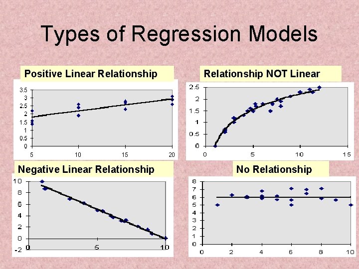
Types of Regression Models Positive Linear Relationship Negative Linear Relationship NOT Linear No Relationship

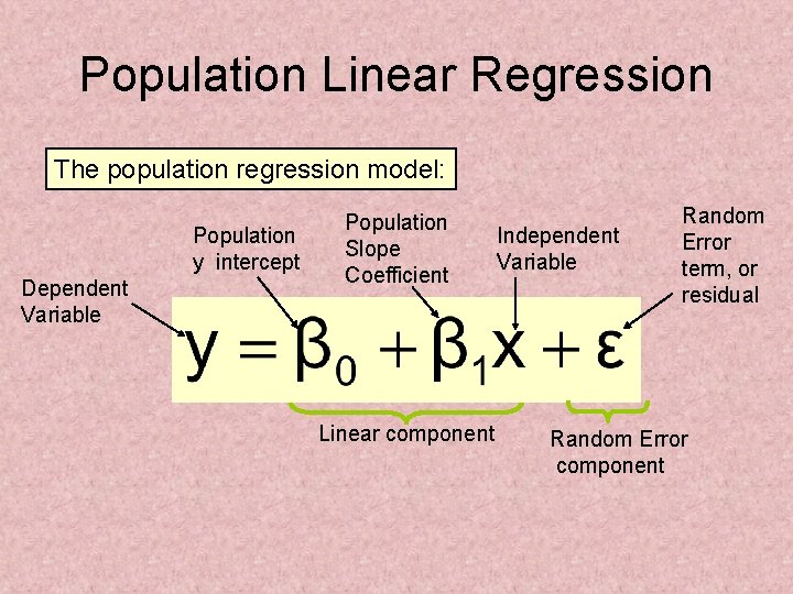
Population Linear Regression The population regression model: Population y intercept Dependent Variable Population Slope Coefficient Linear component Independent Variable Random Error term, or residual Random Error component

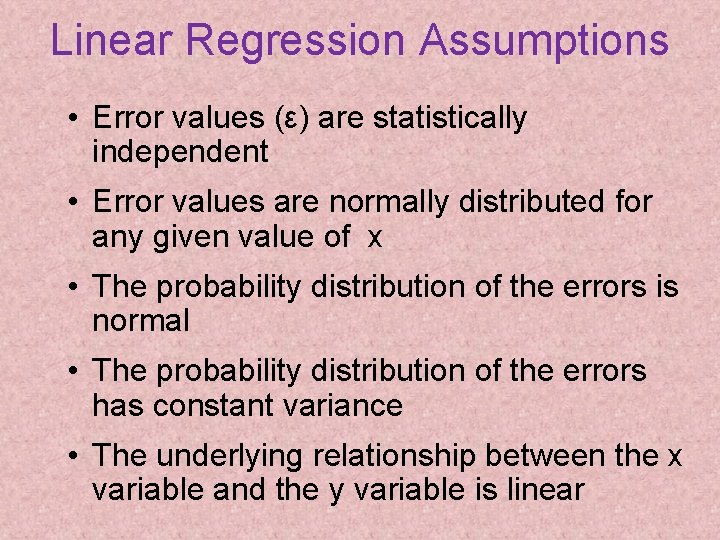
Linear Regression Assumptions • Error values (ε) are statistically independent • Error values are normally distributed for any given value of x • The probability distribution of the errors is normal • The probability distribution of the errors has constant variance • The underlying relationship between the x variable and the y variable is linear

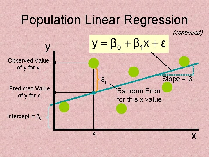
Population Linear Regression (continued) y Observed Value of y for xi εi Predicted Value of y for xi Slope = β 1 Random Error for this x value Intercept = β 0 xi x

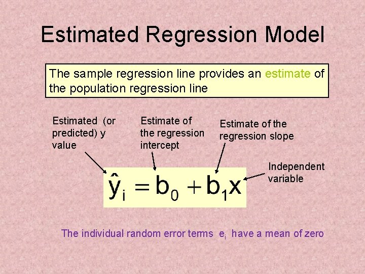
Estimated Regression Model The sample regression line provides an estimate of the population regression line Estimated (or predicted) y value Estimate of the regression intercept Estimate of the regression slope Independent variable The individual random error terms ei have a mean of zero

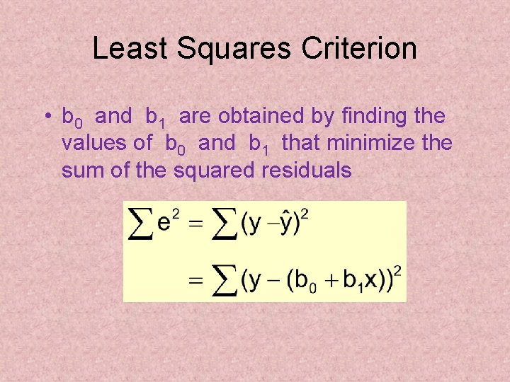
Least Squares Criterion • b 0 and b 1 are obtained by finding the values of b 0 and b 1 that minimize the sum of the squared residuals

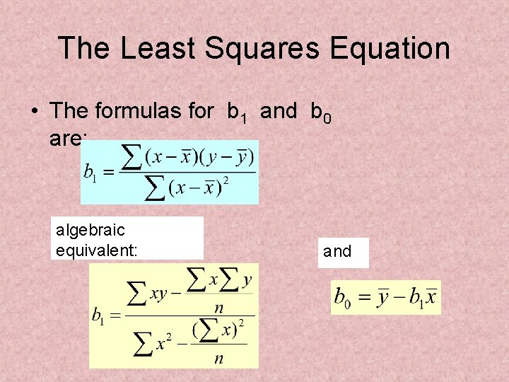
The Least Squares Equation • The formulas for b 1 and b 0 are: algebraic equivalent: and

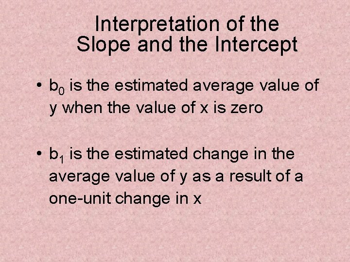
Interpretation of the Slope and the Intercept • b 0 is the estimated average value of y when the value of x is zero • b 1 is the estimated change in the average value of y as a result of a one-unit change in x

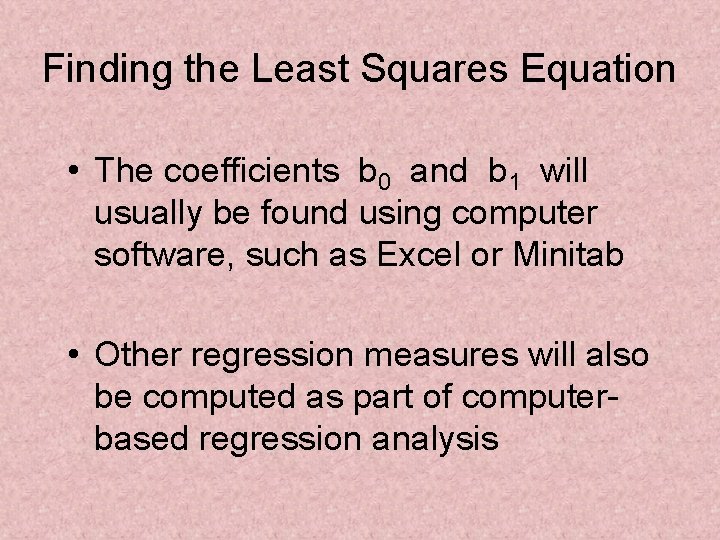
Finding the Least Squares Equation • The coefficients b 0 and b 1 will usually be found using computer software, such as Excel or Minitab • Other regression measures will also be computed as part of computerbased regression analysis

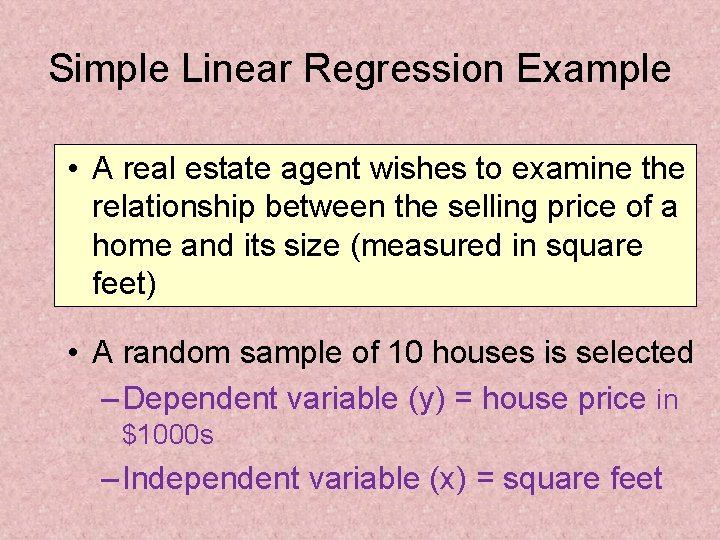
Simple Linear Regression Example • A real estate agent wishes to examine the relationship between the selling price of a home and its size (measured in square feet) • A random sample of 10 houses is selected – Dependent variable (y) = house price in $1000 s – Independent variable (x) = square feet

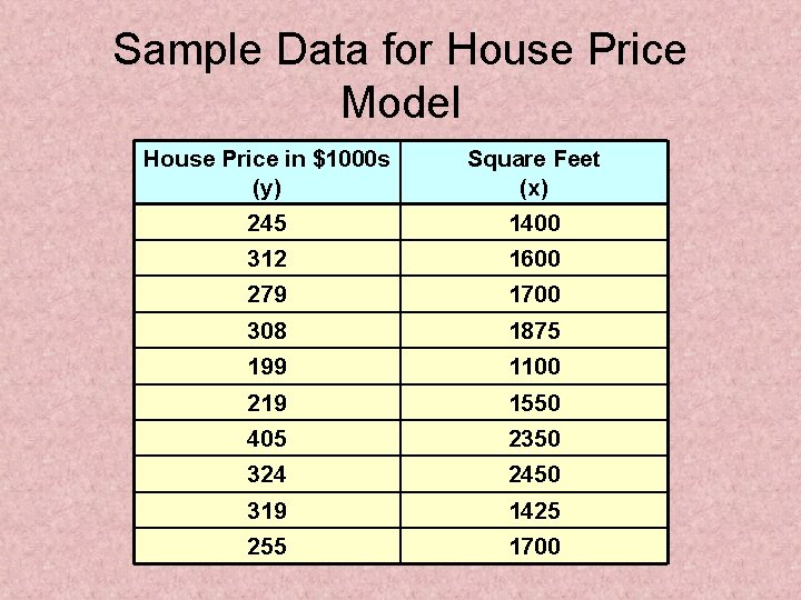
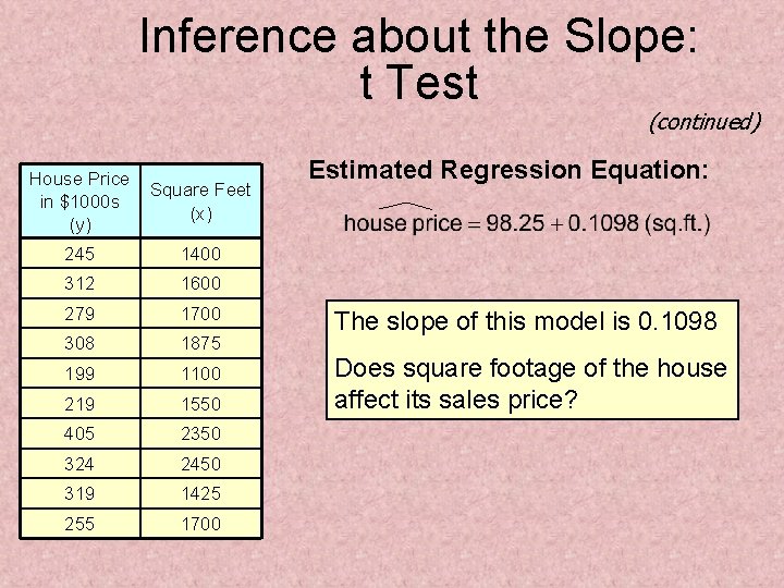
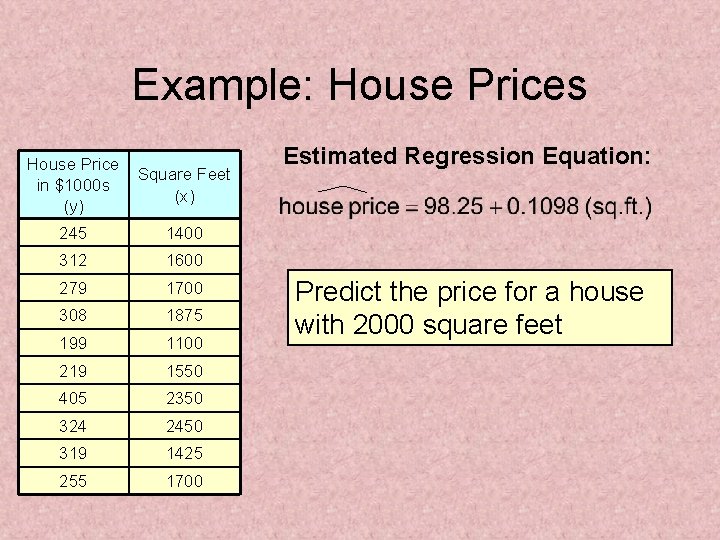
Sample Data for House Price Model House Price in $1000 s (y) 245 Square Feet (x) 1400 312 1600 279 1700 308 1875 199 1100 219 1550 405 2350 324 2450 319 1425 255 1700

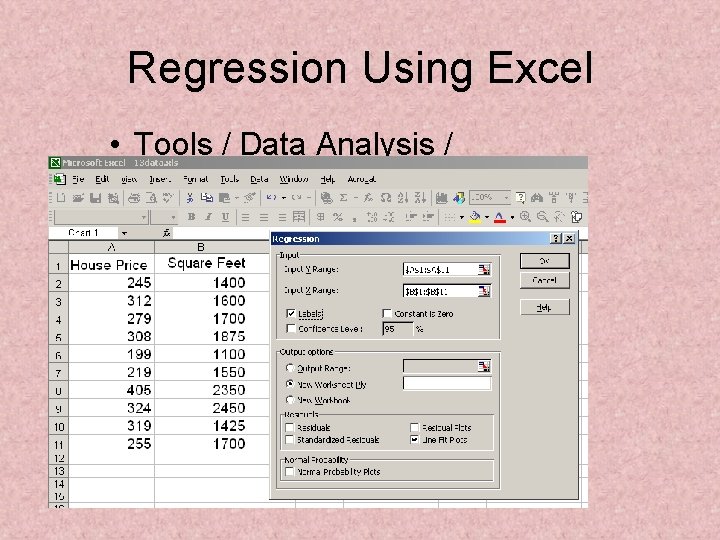
Regression Using Excel • Tools / Data Analysis / Regression

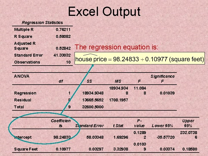
Excel Output Regression Statistics Multiple R 0. 76211 R Square 0. 58082 Adjusted R Square 0. 52842 Standard Error The regression equation is: 41. 33032 Observations 10 ANOVA df SS MS F 11. 084 8 Regression 1 18934. 9348 18934. 934 8 Residual 8 13665. 5652 1708. 1957 Total 9 32600. 5000 Intercept Square Feet Coefficien ts 98. 24833 0. 10977 Standard Error 58. 03348 0. 03297 Significance F 0. 01039 t Stat Pvalue 1. 69296 0. 1289 2 -35. 57720 232. 0738 6 3. 32938 0. 0103 9 0. 03374 0. 18580 Lower 95% Upper 95%

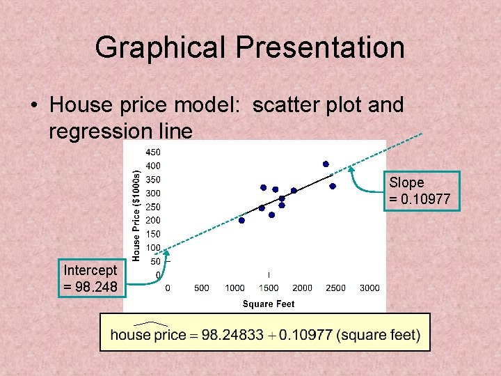
Graphical Presentation • House price model: scatter plot and regression line Slope = 0. 10977 Intercept = 98. 248

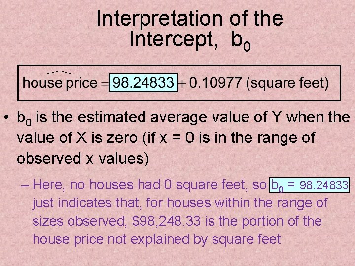
Interpretation of the Intercept, b 0 • b 0 is the estimated average value of Y when the value of X is zero (if x = 0 is in the range of observed x values) – Here, no houses had 0 square feet, so b 0 = 98. 24833 just indicates that, for houses within the range of sizes observed, $98, 248. 33 is the portion of the house price not explained by square feet

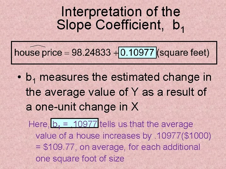
Interpretation of the Slope Coefficient, b 1 • b 1 measures the estimated change in the average value of Y as a result of a one-unit change in X Here, b 1 =. 10977 tells us that the average value of a house increases by. 10977($1000) = $109. 77, on average, for each additional one square foot of size

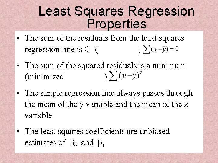
Least Squares Regression Properties • The sum of the residuals from the least squares regression line is 0 ( ) • The sum of the squared residuals is a minimum (minimized ) • The simple regression line always passes through the mean of the y variable and the mean of the x variable • The least squares coefficients are unbiased estimates of β 0 and β 1

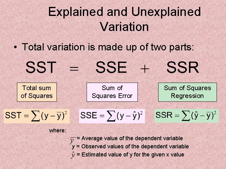
Explained and Unexplained Variation • Total variation is made up of two parts: Total sum of Squares Sum of Squares Error Sum of Squares Regression where: = Average value of the dependent variable y = Observed values of the dependent variable = Estimated value of y for the given x value

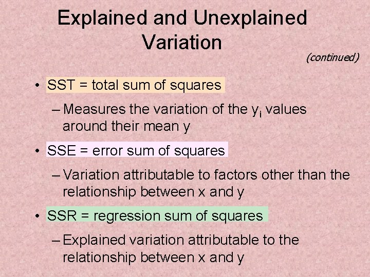
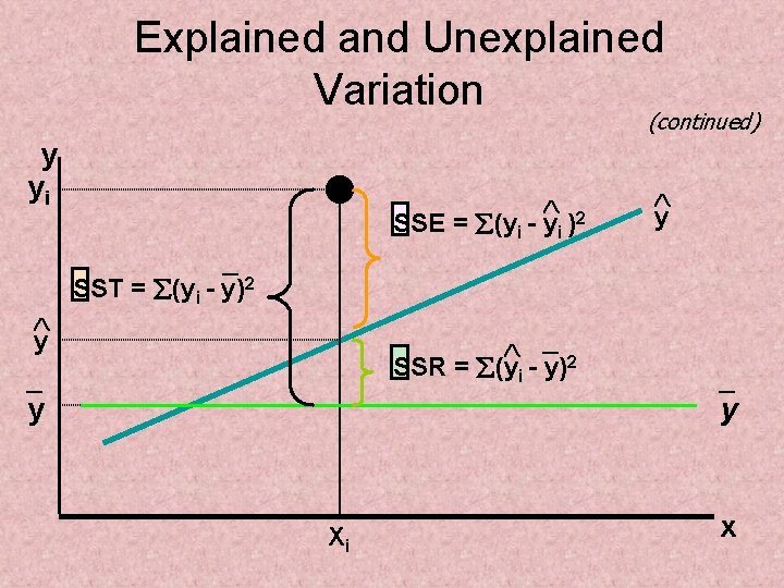
Explained and Unexplained Variation (continued) • SST = total sum of squares – Measures the variation of the yi values around their mean y • SSE = error sum of squares – Variation attributable to factors other than the relationship between x and y • SSR = regression sum of squares – Explained variation attributable to the relationship between x and y

Explained and Unexplained Variation (continued) y yi 2 SSE = (yi - yi ) _ y y SST = (yi - y)2 _2 SSR = (yi - y) _ y Xi _ y x

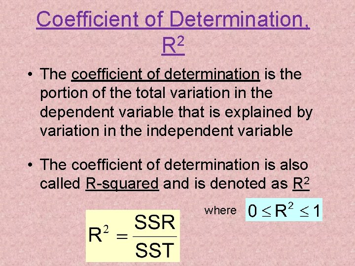
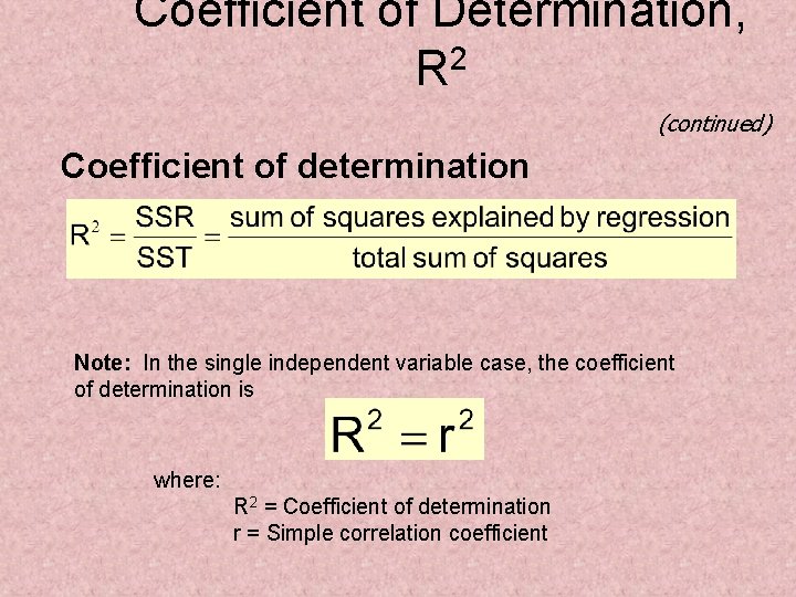
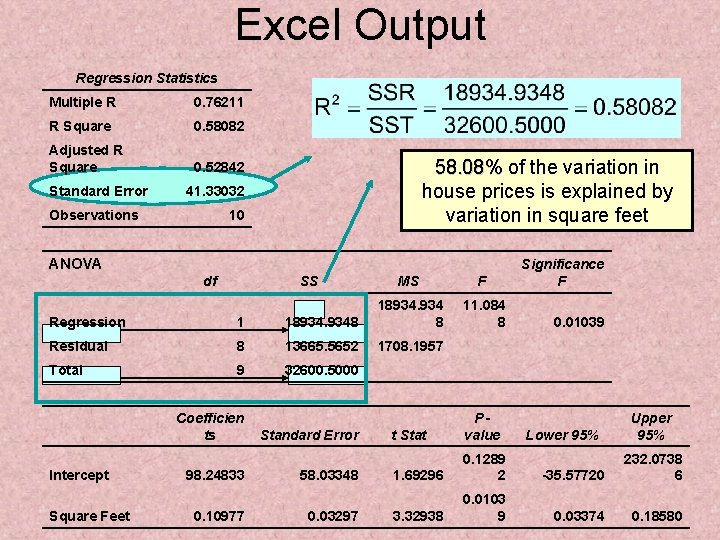
Coefficient of Determination, R 2 • The coefficient of determination is the portion of the total variation in the dependent variable that is explained by variation in the independent variable • The coefficient of determination is also called R-squared and is denoted as R 2 where

Coefficient of Determination, 2 R (continued) Coefficient of determination Note: In the single independent variable case, the coefficient of determination is where: R 2 = Coefficient of determination r = Simple correlation coefficient

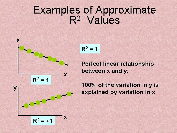
Examples of Approximate R 2 Values y R 2 = 1 x 100% of the variation in y is explained by variation in x y R 2 = +1 Perfect linear relationship between x and y: x

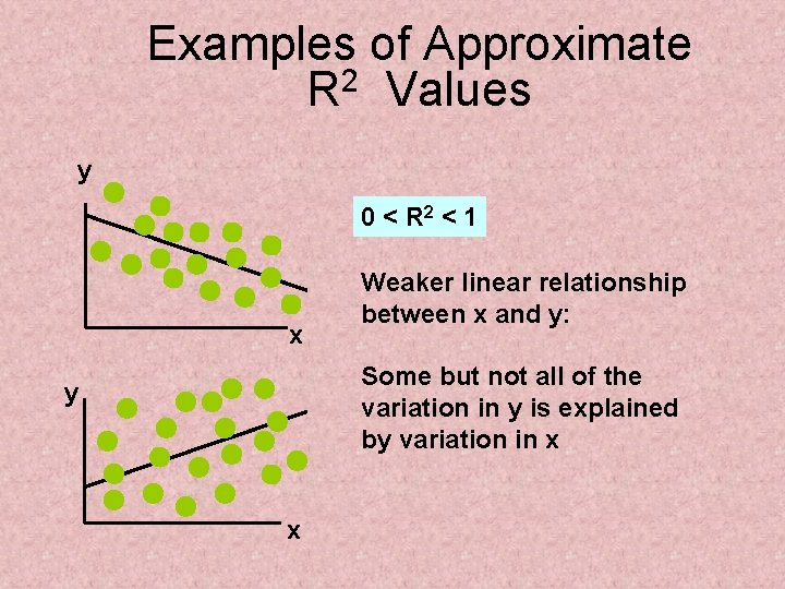
Examples of Approximate R 2 Values y 0 < R 2 < 1 x Weaker linear relationship between x and y: Some but not all of the variation in y is explained by variation in x y x

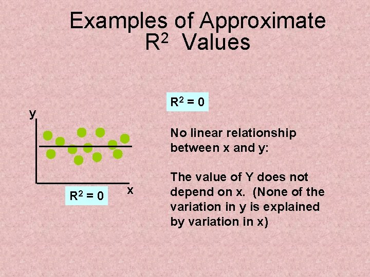
Examples of Approximate R 2 Values R 2 = 0 y No linear relationship between x and y: R 2 = 0 x The value of Y does not depend on x. (None of the variation in y is explained by variation in x)

Excel Output Regression Statistics Multiple R 0. 76211 R Square 0. 58082 Adjusted R Square 0. 52842 Standard Error 58. 08% of the variation in house prices is explained by variation in square feet 41. 33032 Observations 10 ANOVA df SS MS F 11. 084 8 Regression 1 18934. 9348 18934. 934 8 Residual 8 13665. 5652 1708. 1957 Total 9 32600. 5000 Intercept Square Feet Coefficien ts 98. 24833 0. 10977 Standard Error 58. 03348 0. 03297 Significance F 0. 01039 t Stat Pvalue 1. 69296 0. 1289 2 -35. 57720 232. 0738 6 3. 32938 0. 0103 9 0. 03374 0. 18580 Lower 95% Upper 95%

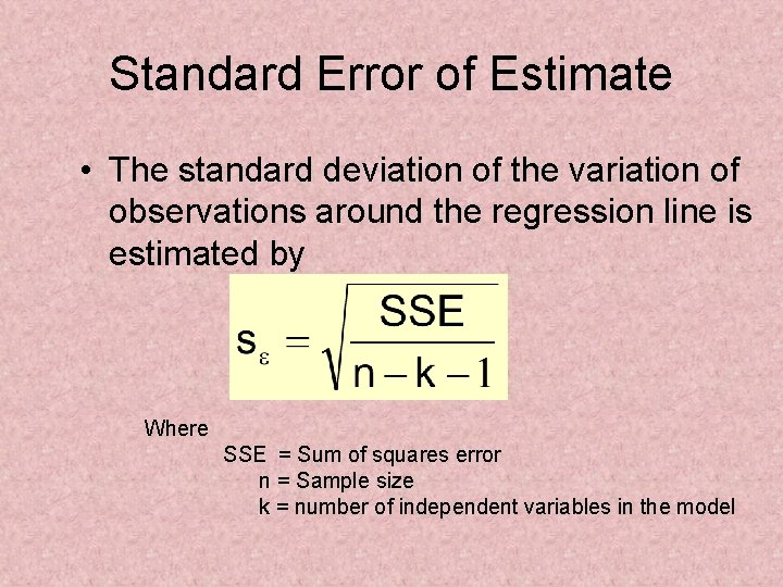
Standard Error of Estimate • The standard deviation of the variation of observations around the regression line is estimated by Where SSE = Sum of squares error n = Sample size k = number of independent variables in the model

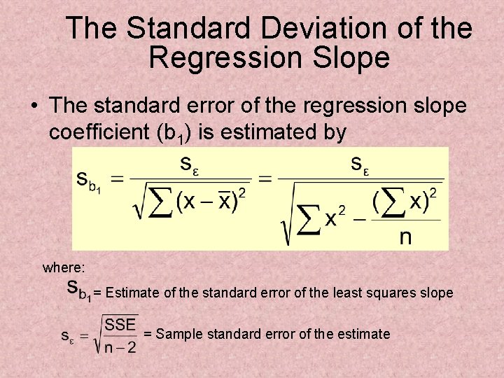
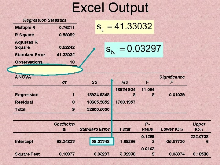
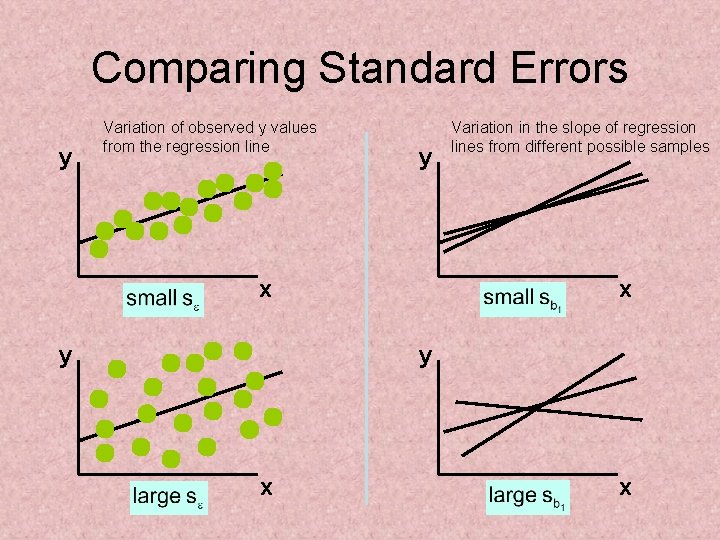
The Standard Deviation of the Regression Slope • The standard error of the regression slope coefficient (b 1) is estimated by where: = Estimate of the standard error of the least squares slope = Sample standard error of the estimate

Excel Output Regression Statistics Multiple R 0. 76211 R Square 0. 58082 Adjusted R Square 0. 52842 Standard Error 41. 33032 Observations 10 ANOVA df SS MS F 11. 084 8 Regression 1 18934. 9348 18934. 934 8 Residual 8 13665. 5652 1708. 1957 Total 9 32600. 5000 Intercept Square Feet Coefficien ts 98. 24833 0. 10977 Standard Error 58. 03348 0. 03297 Significance F 0. 01039 t Stat Pvalue 1. 69296 0. 1289 2 -35. 57720 232. 0738 6 3. 32938 0. 0103 9 0. 03374 0. 18580 Lower 95% Upper 95%

Comparing Standard Errors y Variation of observed y values from the regression line y x y Variation in the slope of regression lines from different possible samples x y x x

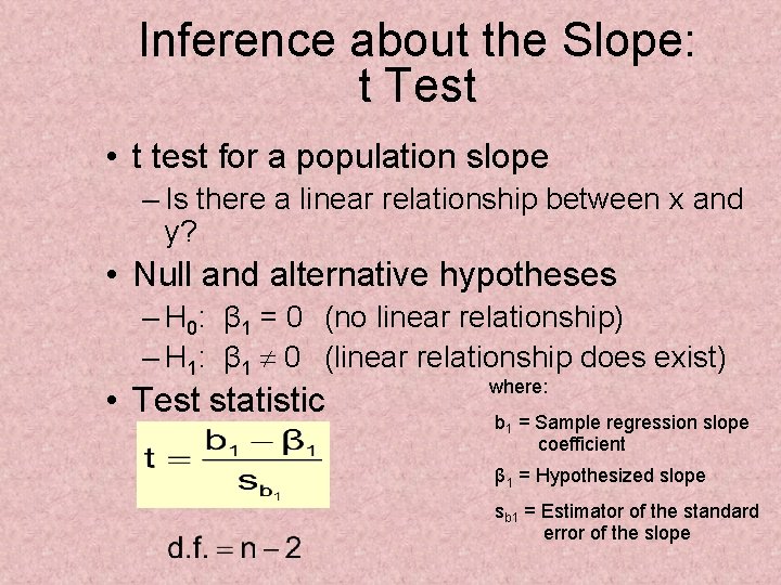
Inference about the Slope: t Test • t test for a population slope – Is there a linear relationship between x and y? • Null and alternative hypotheses – H 0: β 1 = 0 (no linear relationship) – H 1: β 1 0 (linear relationship does exist) • Test statistic – where: b 1 = Sample regression slope coefficient β 1 = Hypothesized slope sb 1 = Estimator of the standard error of the slope

Inference about the Slope: t Test (continued) House Price in $1000 s (y) Square Feet (x) 245 1400 312 1600 279 1700 308 1875 199 1100 219 1550 405 2350 324 2450 319 1425 255 1700 Estimated Regression Equation: The slope of this model is 0. 1098 Does square footage of the house affect its sales price?

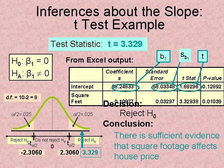
Inferences about the Slope: t Test Example Test Statistic: t = 3. 329 From Excel output: H 0: β 1 = 0 HA : β 1 0 Intercept Square Feet d. f. = 10 -2 = 8 a/2=. 025 Reject H 0 a/2=. 025 Do not reject H 0 -tα/2 -2. 3060 0 Reject H 0 tα/2 2. 3060 3. 329 Coefficient s 98. 24833 b 1 Standard Error t t Stat P-value 58. 03348 1. 69296 0. 12892 0. 10977 0. 03297 3. 32938 0. 01039 Decision: Reject H 0 Conclusion: There is sufficient evidence that square footage affects house price

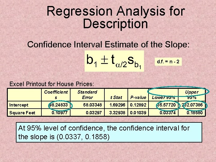
Regression Analysis for Description Confidence Interval Estimate of the Slope: d. f. = n - 2 Excel Printout for House Prices: Intercept Square Feet Coefficient s Standard Error t Stat P-value Lower 95% Upper 95% 98. 24833 58. 03348 1. 69296 0. 12892 -35. 57720 232. 07386 0. 10977 0. 03297 3. 32938 0. 01039 0. 03374 0. 18580 At 95% level of confidence, the confidence interval for the slope is (0. 0337, 0. 1858)

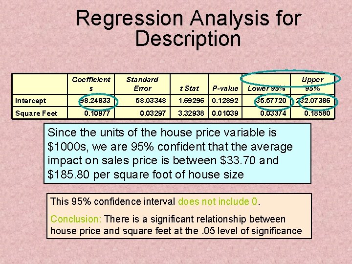
Regression Analysis for Description Coefficient s Intercept Square Feet Standard Error t Stat P-value Lower 95% Upper 95% 98. 24833 58. 03348 1. 69296 0. 12892 -35. 57720 232. 07386 0. 10977 0. 03297 3. 32938 0. 01039 0. 03374 0. 18580 Since the units of the house price variable is $1000 s, we are 95% confident that the average impact on sales price is between $33. 70 and $185. 80 per square foot of house size This 95% confidence interval does not include 0. Conclusion: There is a significant relationship between house price and square feet at the. 05 level of significance

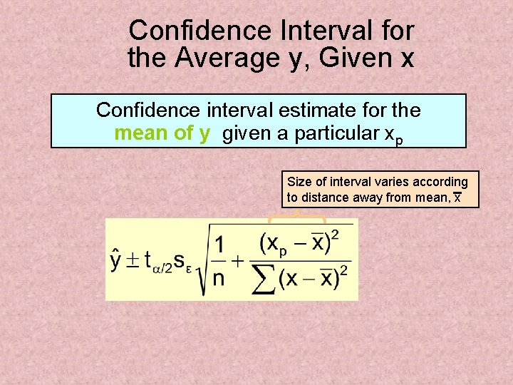
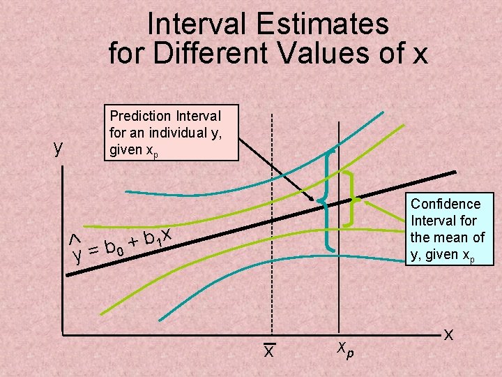
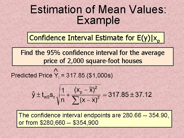
Confidence Interval for the Average y, Given x Confidence interval estimate for the mean of y given a particular xp Size of interval varies according to distance away from mean, x

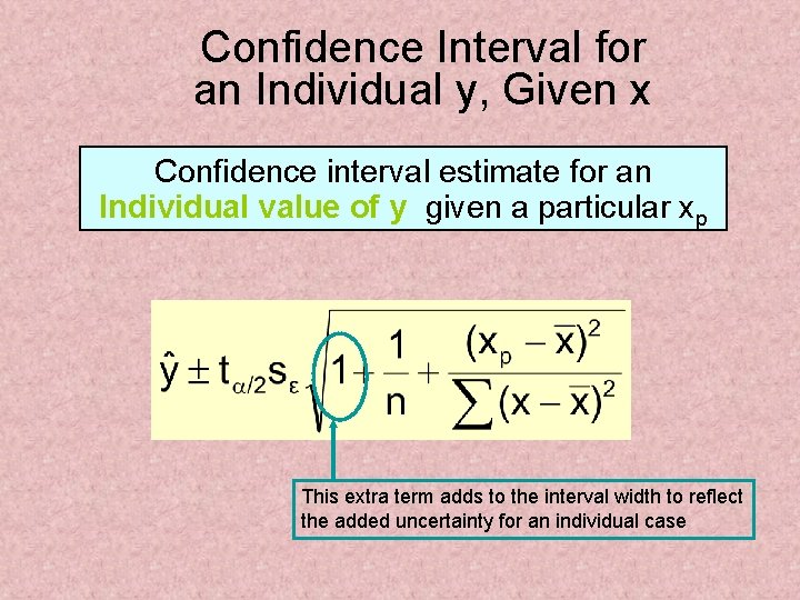
Confidence Interval for an Individual y, Given x Confidence interval estimate for an Individual value of y given a particular xp This extra term adds to the interval width to reflect the added uncertainty for an individual case

Interval Estimates for Different Values of x y Prediction Interval for an individual y, given xp Confidence Interval for the mean of y, given xp b 1 x + y = b 0 x xp x

Example: House Prices House Price in $1000 s (y) Square Feet (x) 245 1400 312 1600 279 1700 308 1875 199 1100 219 1550 405 2350 324 2450 319 1425 255 1700 Estimated Regression Equation: Predict the price for a house with 2000 square feet

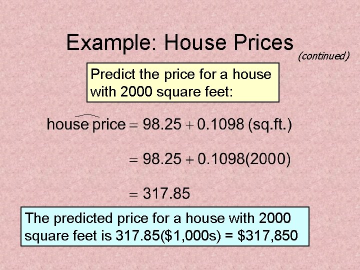
Example: House Prices (continued) Predict the price for a house with 2000 square feet: The predicted price for a house with 2000 square feet is 317. 85($1, 000 s) = $317, 850

Estimation of Mean Values: Example Confidence Interval Estimate for E(y)|xp Find the 95% confidence interval for the average price of 2, 000 square-foot houses Predicted Price Yi = 317. 85 ($1, 000 s) The confidence interval endpoints are 280. 66 -- 354. 90, or from $280, 660 -- $354, 900

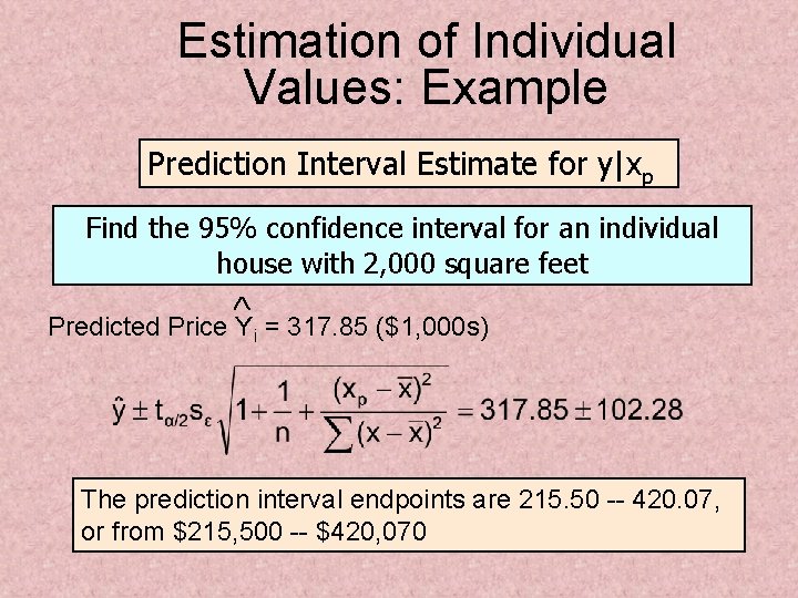
Estimation of Individual Values: Example Prediction Interval Estimate for y|xp Find the 95% confidence interval for an individual house with 2, 000 square feet Predicted Price Yi = 317. 85 ($1, 000 s) The prediction interval endpoints are 215. 50 -- 420. 07, or from $215, 500 -- $420, 070

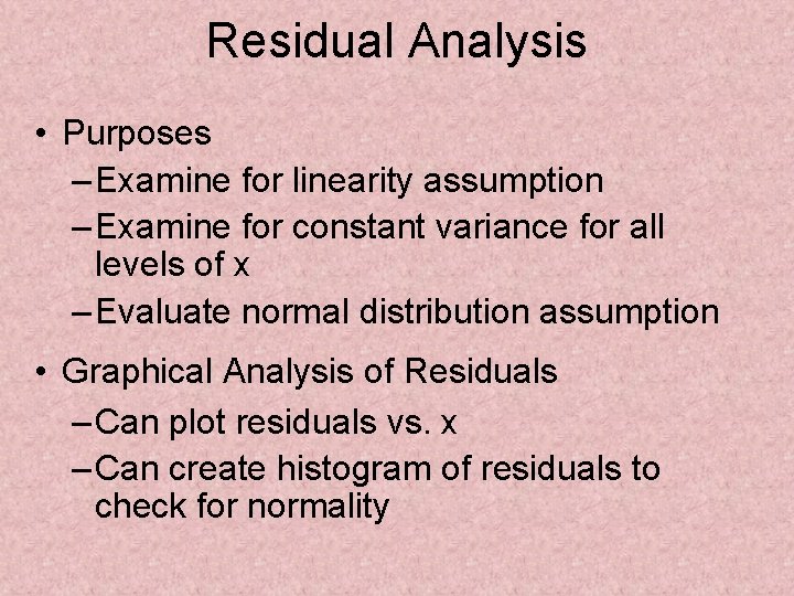
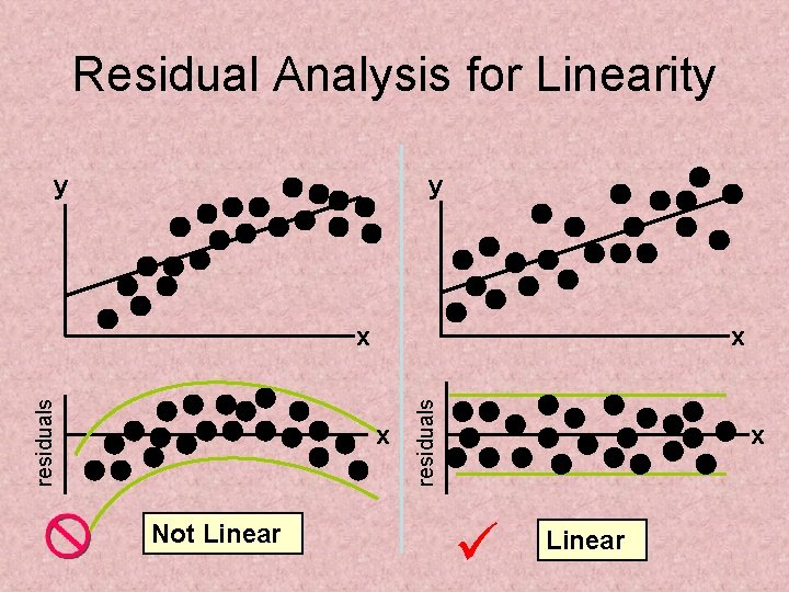
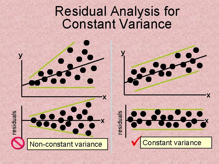
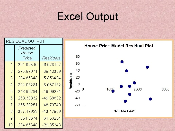
Residual Analysis • Purposes – Examine for linearity assumption – Examine for constant variance for all levels of x – Evaluate normal distribution assumption • Graphical Analysis of Residuals – Can plot residuals vs. x – Can create histogram of residuals to check for normality

Residual Analysis for Linearity y y x x Not Linear residuals x x Linear

Residual Analysis for Constant Variance y y x x Non-constant variance residuals x x Constant variance

Excel Output RESIDUAL OUTPUT Predicted House Price Residuals 1 251. 92316 -6. 923162 2 273. 87671 38. 12329 3 284. 85348 -5. 853484 4 304. 06284 3. 937162 5 218. 99284 -19. 99284 6 268. 38832 -49. 38832 7 356. 20251 48. 79749 8 367. 17929 -43. 17929 9 254. 6674 64. 33264 10 284. 85348 -29. 85348

Summary • Introduced correlation analysis • Discussed correlation to measure the strength of a linear association • Introduced simple linear regression analysis • Calculated the coefficients for the simple linear regression equation • measures of variation (R 2 and sε) • Addressed assumptions of regression and correlation

Summary (continued) • Described inference about the slope • Addressed estimation of mean values and prediction of individual values • Discussed residual analysis

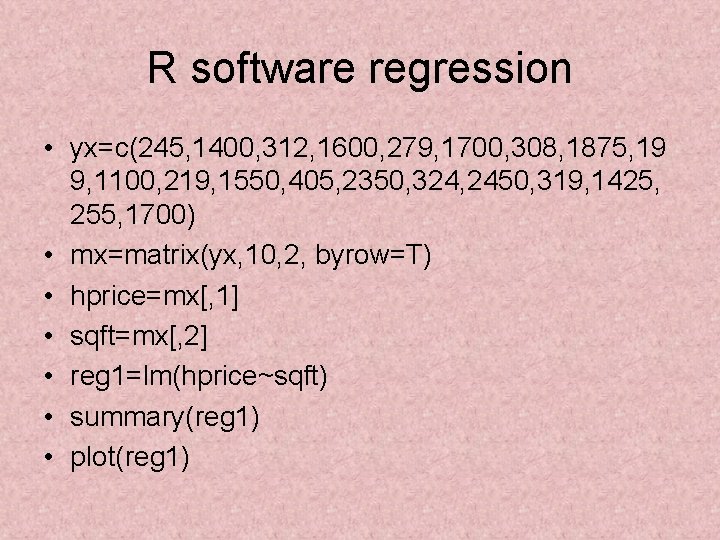
R software regression • yx=c(245, 1400, 312, 1600, 279, 1700, 308, 1875, 19 9, 1100, 219, 1550, 405, 2350, 324, 2450, 319, 1425, 255, 1700) • mx=matrix(yx, 10, 2, byrow=T) • hprice=mx[, 1] • sqft=mx[, 2] • reg 1=lm(hprice~sqft) • summary(reg 1) • plot(reg 1)