Introduction to Linear Programming Source 1 Operations Research

Introduction to Linear Programming Source: 1. Operations Research: Applications & Algorithms, 4 th edition, by Wayne L. Winston 2. Jim Orlin Power. Point presentation 1

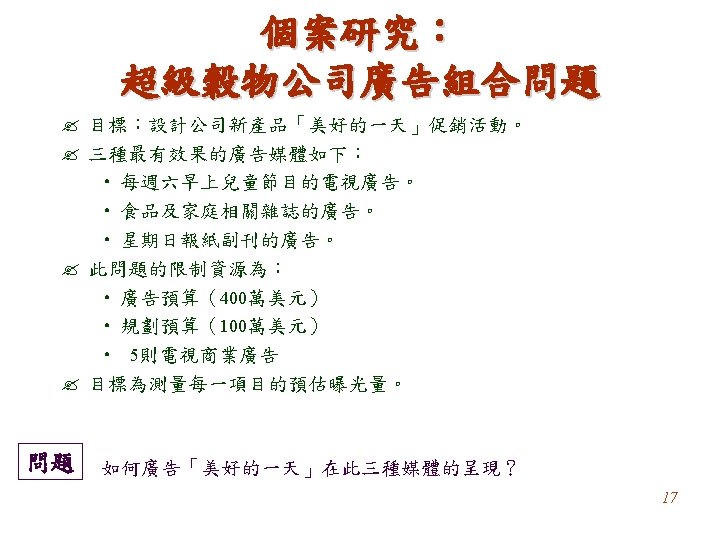
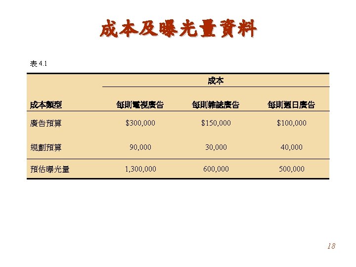
What Is a Linear Programming Problem? Example Giapetto’s, Inc. , manufactures wooden soldiers and trains. Each soldier built: • Sell for $27 and uses $10 worth of raw materials. • Increase Giapetto’s variable labor/overhead costs by $14. • Requires 2 hours of finishing labor. • Requires 1 hour of carpentry labor. Each train built: • Sell for $21 and used $9 worth of raw materials. • Increases Giapetto’s variable labor/overhead costs by $10. • Requires 1 hour of finishing labor. • Requires 1 hour of carpentry labor. 2

What Is a Linear Programming Problem? Each week Giapetto can obtain: • All needed raw material. • Only 100 finishing hours. • Only 80 carpentry hours. Also: • Demand for the trains is unlimited. • At most 40 soldiers are bought each week. Giapetto wants to maximize weekly profit (revenues – expenses). Formulate a mathematical model of Giapetto’s situation that can be used maximize weekly profit. 3

What Is a Linear Programming Problem? The Giapetto solution model incorporates the characteristics shared by all linear programming problems. Decision Variables x 1 = number of soldiers produced each week x 2 = number of trains produced each week Objective Function In any linear programming model, the decision maker wants to maximize (usually revenue or profit) or minimize (usually costs) some function of the decision variables. This function to maximized or minimized is called the objective function. For the Giapetto problem, fixed costs are do not depend upon the values of x 1 or x 2. 4

What Is a Linear Programming Problem? Giapetto’s weekly profit can be expressed in terms of the decision variables x 1 and x 2: Weekly profit = weekly revenue – weekly raw material costs – the weekly variable costs Weekly revenue = 27 x 1 + 21 x 2 Weekly raw material costs = 10 x 1 + 9 x 2 Weekly variable costs = 14 x 1 + 10 x 2 Weekly profit = (27 x 1 + 21 x 2) – (10 x 1 + 9 x 2) – (14 x 1 + 10 x 2 ) = 3 x 1 + 2 x 2 5

What Is a Linear Programming Problem? Giapetto’s objective is to chose x 1 and x 2 to maximize 3 x 1 + 2 x 2. We use the variable z to denote the objective function value of any LP. Giapetto’s objective function is: Maximize z = 3 x 1 + 2 x 2 “Maximize” will be abbreviated by max and “minimize” by min. The coefficient of an objective function variable is called an objective function coefficient. 6

What Is a Linear Programming Problem? Constraints: As x 1 and x 2 increase, Giapetto’s objective function grows larger. For Giapetto, the values of x 1 and x 2 are limited by the following three restrictions (often called constraints): Constraint 1 Each week, no more than 100 hours of finishing time may be used. Constraint 2 Each week, no more than 80 hours of carpentry time may be used. Constraint 3 Because of limited demand, at most 40 soldiers should be produced. These three constraints can be expressed mathematically by the following equations: Constraint 1: 2 x 1 + x 2 ≤ 100 Constraint 2: x 1 + x 2 ≤ 80 Constraint 3: x 1 ≤ 40 7

What Is a Linear Programming Problem? For the Giapetto problem model, combining the sign restrictions x 1 ≥ 0 and x 2 ≥ 0 with the objective function and constraints yields the following optimization model: Max z = 3 x 1 + 2 x 2 (objective function) Subject to (s. t. ) 2 x 1 + x 2 ≤ 100 (finishing constraint) x 1 + x 2 ≤ 80 (carpentry constraint) x 1 ≤ 40 (constraint on demand for soldiers) x 1 ≥ 0 (sign restriction) x 2 8

What Is a Linear Programming Problem? Concepts of linear function and linear inequality: Linear Function: A function f(x 1, x 2, …, xn of x 1, x 2, …, xn is a linear function if and only if for some set of constants, c 1, c 2, …, cn, f(x 1, x 2, …, xn) = c 1 x 1 + c 2 x 2 + … + cnxn. For example, f(x 1, x 2) = 2 x 1 + x 2 is a linear function of x 1 and x 2, but f(x 1, x 2) = (x 1)2 x 2 is not a linear function of x 1 and x 2. For any linear function f(x 1, x 2, …, xn) and any number b, the inequalities inequality f(x 1, x 2, …, xn) £ b and f(x 1, x 2, …, xn) b are linear inequalities. 9

What Is a Linear Programming Problem? A linear programming problem (LP) is an optimization problem for which we do the following: 1. Attempt to maximize (or minimize) a linear function (called the objective function) of the decision variables. 2. The values of the decision variables must satisfy a set of constraints. Each constraint must be a linear equation or inequality. 3. A sign restriction is associated with each variable. For each variable xi, the sign restriction specifies either that xi must be nonnegative (xi ≥ 0) or that xi may be unrestricted in sign. 10

What Is a Linear Programming Problem? Proportionality and Additive Assumptions The objective function for an LP must be a linear function of the decision variables has two implications: 1. The contribution of the objective function from each decision variable is proportional to the value of the decision variable. For example, the contribution to the objective function for 4 soldiers is exactly fours times the contribution of 1 soldier. 2. The contribution to the objective function for any variable is independent of the other decision variables. For example, no matter what the value of x 2, the manufacture of x 1 soldiers will always contribute 3 x 1 dollars to the objective function. 11

What Is a Linear Programming Problem? Each LP constraint must be a linear inequality or linear equation has two implications: 1. The contribution of each variable to the left-hand side of each constraint is proportional to the value of the variable. For example, it takes exactly 3 times as many finishing hours to manufacture 3 soldiers as it does 1 soldier. 2. The contribution of a variable to the left-hand side of each constraint is independent of the values of the variable. For example, no matter what the value of x 1, the manufacture of x 2 trains uses x 2 finishing hours and x 2 carpentry hours 12

What Is a Linear Programming Problem? Divisibility Assumption The divisibility assumption requires that each decision variable be permitted to assume fractional values. For example, this assumption implies it is acceptable to produce a fractional number of trains. The Giapetto LP does not satisfy the divisibility assumption since a fractional soldier or train cannot be produced. The use of integer programming methods necessary to address the solution to this problem. The Certainty Assumption The certainty assumption is that each parameter (objective function coefficients, right-hand side, and technological coefficients) are known with certainty. 13

What Is a Linear Programming Problem? Feasible Region and Optimal Solution The feasible region of an LP is the set of all points satisfying all the LP’s constraints and sign restrictions. x 1 = 40 and x 2 = 20 are in the feasible region since they satisfy all the Giapetto constraints. On the other hand, x 1 = 15, x 2 = 70 is not in the feasible region because this point does not satisfy the carpentry constraint [15 + 70 is > 80]. Giapetto Constraints 2 x 1 + x 2 ≤ 100 (finishing constraint) x 1 + x 2 ≤ 80 (carpentry constraint) x 1 ≤ 40 (demand constraint) x 1 ≥ 0 (sign restriction) x 2 ≥ 0 (sign restriction) 14

What Is a Linear Programming Problem? For a maximization problem, an optimal solution to an LP is a point in the feasible region with the largest objective function value. Similarly, for a minimization problem, an optimal solution is a point in the feasible region with the smallest objective function value. Most LPs have only one optimal solution. However, some LPs have no optimal solution, and some LPs have an infinite number of solutions. The optimal solution to the Giapetto LP is x 1 = 20 and x 2 = 60. This solution yields an objective function value of: z = 3 x 1 + 2 x 2 = 3(20) + 2(60) = $180 When we say x 1 = 20 and x 2 = 60 is the optimal solution, we are saying that no point in the feasible region has an objective function value (profit) exceeding 180. 15

More Linear Programming Models 16

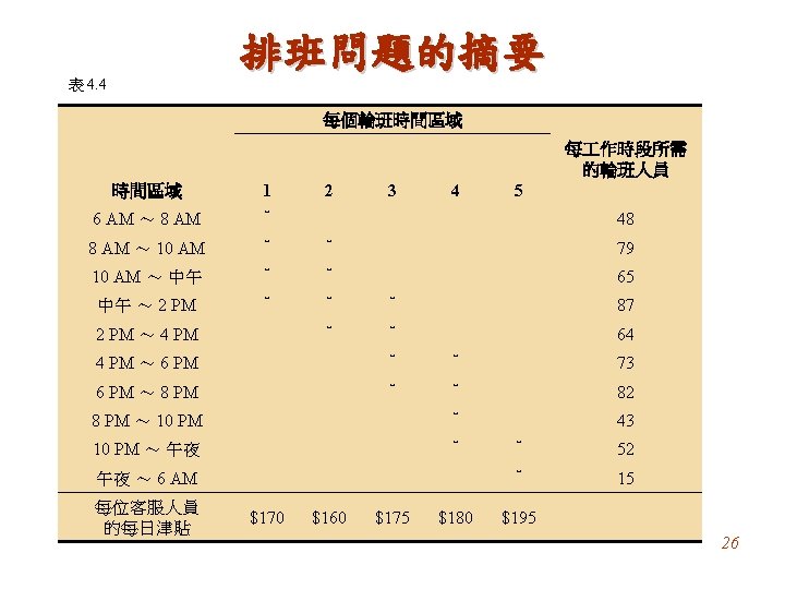
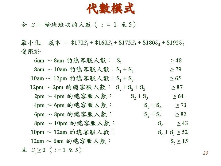
試算表模式 B C D E F G 3 6 am-2 pm 8 am-4 pm 中午-8 pm 4 pm-午夜 10 pm-6 am 4 時段 時段 時段 $170 $160 $175 $180 $195 5 每一輪班成 本 6 7 輪班時段 (1=yes, 0=no) H I J 總 最低 人數 需求 8 6 am-8 am 1 0 0 48 ≥ 48 9 8 am-10 am 1 1 0 0 0 79 ≥ 79 10 10 am- 12 pm 1 1 0 0 0 79 ≥ 65 11 12 pm-2 pm 1 1 1 0 0 118 ≥ 87 12 2 pm-4 pm 0 1 1 0 0 70 ≥ 64 13 4 pm-6 pm 0 0 1 1 0 82 ≥ 73 14 6 pm-8 pm 0 0 1 1 0 82 ≥ 82 15 8 pm-10 pm 0 0 0 1 0 43 ≥ 43 16 10 pm-12 am 0 0 0 1 1 58 ≥ 52 17 12 am-6 am 0 0 1 15 ≥ 15 19 6 am-2 pm 8 am-4 pm 中午-8 pm 4 pm-午夜 10 pm-6 am 20 時段 時段 時段 總成本 48 31 39 43 15 $30, 610 圖 4. 3 18 21 員 人數 27

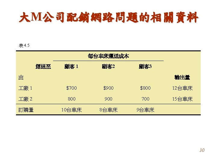
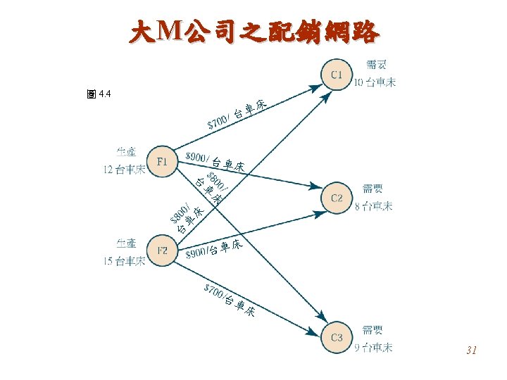
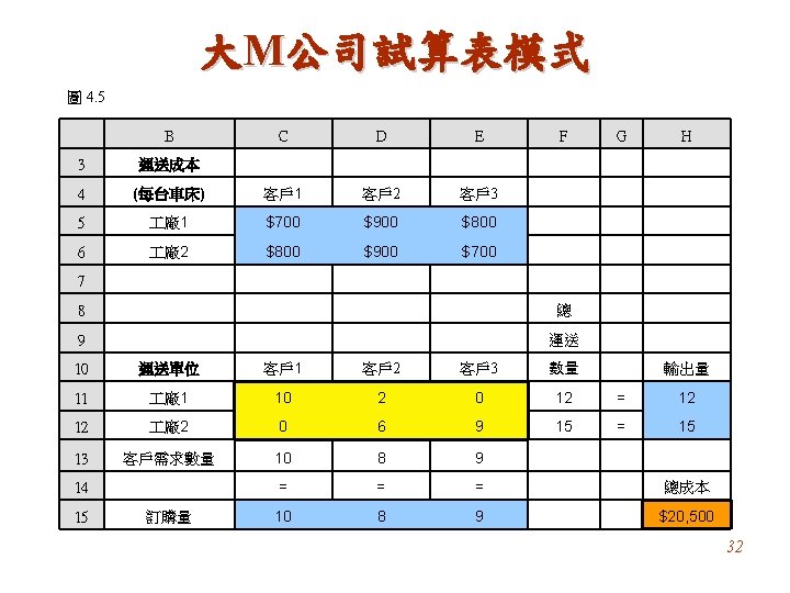
大M公司代數模式 令 Sij = 從 i 到 j運送車床的數量（i = F 1, F 2； j = C 1, C 2, C 3） 最小化 成本 = $700 SF 1 -C 1 + $900 SF 1 -C 2 + $800 SF 1 -C 3 + $800 SF 2 -C 1 + $900 SF 2 -C 2 + $700 SF 2 -C 3 受限於 廠 廠 客戶 客戶 客戶 且 1：SF 1 -C 1 + SF 1 -C 2 + SF 1 -C 3 = 12 2： SF 2 -C 1 + SF 2 -C 2 + SF 2 -C 3 = 15 1：SF 1 -C 1 + SF 2 -C 1 = 10 2： SF 1 -C 2 + SF 2 -C 2 = 8 3： SF 1 -C 3 + SF 2 -C 3 = 9 Sij ≥ 0（i = F 1, F 2；j = C 1, C 2, C 3） 33

Scheduling Postal Workers • • Each postal worker works for 5 consecutive days, followed by 2 days off, repeated weekly. Minimize the number of postal workers (for the time being, we will permit fractional workers on each day. ) 44

Formulating as an LP • Select the decision variables – Let x 1 be the number of workers who start working on Monday, and work till Friday – Let x 2 be the number of workers who start on Tuesday … – Let x 3, x 4, …, x 7 be defined similarly. 45

The linear program Minimize z = x 1 + x 2 + x 3 + x 4 + x 5 + x 6 + x 7 subject to x 1 + x 4 + x 5 + x 6 + x 7 17 x 1 + x 2 + x 5 + x 6 + x 7 13 x 1 + x 2 + x 3 + x 6 + x 7 15 x 1 + x 2 + x 3 + x 4 + x 7 19 x 1 + x 2 + x 3 + x 4 + x 5 14 x 2 + x 3 + x 4 + x 5 + x 6 16 x 3 + x 4 + x 5 + x 6 + x 7 11 xj 0 for j = 1 to 7 46

Minimize z = x 1 + x 2 + x 3 + x 4 + x 5 + x 6 + x 7 subject to x 1 + x 4 + x 5 + x 6 + x 7 - s 1 x 1 + x 2 + x 5 + x 6 + x 7 - s 2 x 1 + x 2 + x 3 + x 6 + x 7 - s 3 x 1 + x 2 + x 3 + x 4 + x 7 - s 4 x 1 + x 2 + x 3 + x 4 + x 5 s 5 x 2 + x 3 + x 4 + x 5 + x 6 - s 6 x 3 + x 4 + x 5 + x 6 + x 7 - s 7 xj 0 , sj 0 = 17 = 13 = 15 = 19 = 14 = 16 = 11 for j = 1 to 7 47

A non-linear objective that often can be made linear. Suppose that one wants to minimize the maximum of the slacks, that is minimize z = max (s 1, s 2, …, s 7). This is a non-linear objective. But we can transform it, so the problem becomes an LP. 48

Minimize z z sj subject to for j = 1 to 7. x 1 + x 4 + x 5 + x 6 + x 7 - s 1 x 1 + x 2 + x 5 + x 6 + x 7 - s 2 x 1 + x 2 + x 3 + x 6 + x 7 - s 3 x 1 + x 2 + x 3 + x 4 + x 7 - s 4 x 1 + x 2 + x 3 + x 4 + x 5 s 5 x 2 + x 3 + x 4 + x 5 + x 6 - s 6 x 3 + x 4 + x 5 + x 6 + x 7 - s 7 xj 0 , sj 0 = 17 = 13 = 15 = 19 = 14 = 16 = 11 for j = 1 to 7 The new constraint ensures that z max (s 1, …, s 7) The objective ensures that z = sj for some j. 49

Non-linear objective that often can be made linear. Suppose that the “goal” is to have dj workers on day j. Let yj be the number of workers on day j. Suppose that the objective is minimize Si | yj – d j | This is a non-linear objective. But we can transform it, so the problem becomes an LP. 50

Minimize subject to Sj zj zj dj - yj for j = 1 to 7. zj yj - dj for j = 1 to 7. x 1 + x 4 + x 5 + x 6 + x 7 = y 1 x 1 + x 2 + x 5 + x 6 + x 7 = y 2 x 1 + x 2 + x 3 + x 6 + x 7 = y 3 x 1 + x 2 + x 3 + x 4 + x 7 = y 4 x 1 + x 2 + x 3 + x 4 + x 5 = y 5 x 2 + x 3 + x 4 + x 5 + x 6 = y 6 x 3 + x 4 + x 5 + x 6 + x 7 = y 7 xj 0 , yj 0 for j = 1 to 7 The new constraints ensure that zj | yj – dj | for each j. The objective ensures that zj = | yj – dj | for each j. 51

A ratio constraint: Suppose that we need to ensure that at least 30% of the workers have Sunday off. How do we model this? (x 1 + x 2 )/x 1 + x 2 + x 3 + x 4 + x 5 + x 6 + x 7 . 3 (x 1 + x 2 ) . 3 x 1 +. 3 x 2 +. 3 x 3 +. 3 x 4 +. 3 x 5 +. 3 x 6 +. 3 x 7 -. 7 x 1 -. 7 x 2 +. 3 x 3 +. 3 x 4 +. 3 x 5 +. 3 x 6 +. 3 x 7 <= 0 52

Cost per Ounce and Dietary Requirements for Diet Problem 53

Example 4 -2 Diet Problem 54

Example 4 -3 Blending Problem Formulate the appropriate model for the following blending problem: The sugar content of three juices— orange, banana, and pineapple—is 10, 15, and 20 percent, respectively. How many quarts of each must be mixed together to achieve one gallon (four quarts) that has a sugar content of at least 17 percent to minimize cost? The cost per quart is 20 cents for orange juice, 30 cents for banana juice, and 40 cents for pineapple juice. Solution Variable definitions O = quantity of orange juice in quarts B = quantity of banana juice in quarts P = quantity of pineapple juice in quarts 55

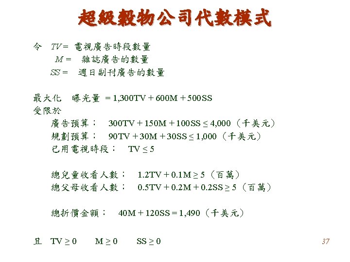
Example 4 -5 Media Selection The Long Last Appliance Sales Company is in the business of selling appliances such as microwave ovens, traditional ovens, refrigerators, dishwashers, dryers, and the like. The company has stores in the greater Chicagoland area and has a monthly advertising budget of $90, 000. Among its options are radio advertising, advertising in the cable TV channels, newspaper advertising, and direct-mail advertising. A 30 -second advertising spot on the local cable channel costs $1, 800, a 30 -second radio ad costs $350, a half-page ad in the local newspaper costs $700, and a single mailing of direct-mail insertion for the entire region costs $1, 200 per mailing. The number of potential buying customers reached per advertising medium usage is as follows: Radio TV Newspaper Direct mail 7, 000 50, 000 18, 000 34, 000 Due to company restrictions and availability of media, the maximum number of usages of each medium is limited to the following: Radio TV 2 Newspaper Direct mail 35 5 30 18 56

Example 4 -5 (cont’d) The management of the company has met and decided that in order to ensure a balanced utilization of different types of media and to portray a positive image of the company, at least 10 percent of the advertisements must be on TV. No more than 40 percent of the advertisements must be on radio. The cost of advertising allocated to TV and direct mail cannot exceed 60 percent of the total advertising budget. What is the optimal allocation of the budget among the four media? What is the total maximum audience contact? 57

Example 4 -5 (cont’d) 58

Marketing Research • Stages of marketing research study development: – Design study. – Conduct marketing survey. – Analyze data and obtain results. – Make recommendations based on the results. 59

Example 4 -6 Market Research Market Facts Inc. is a marketing research firm that works with client companies to determine consumer reaction toward various products and services. A client company requested that Market Facts investigate the consumer reaction to a recently developed electronic device. Market Facts and the client company agreed that a combination of telephone interviews and direct-mail questionnaires would be used to obtain the information from different type of households. The households are divided into six categories: 1. Households containing a single person under 40 years old and without children under 18 years of age. 2. Households containing married people under 40 years old and without children under 18 years of age. 3. Households containing single parents with children under 18 years of age. 4. Households containing married families with children under 18 years of age. 5. Households containing single people over 40 years old without children under 18 years of age. 6. Households containing married people over 40 years old without children under 18 years of age. 60

Example 4 -6 (cont’d) Restrictions 1. At least 60 percent of the phone interviews must be conducted at households with children. 2. At least 50 percent of the direct-mail questionnaires must be mailed to households with children. 3. No more than 30 percent of the phone interviews and mail-in questionnaires must be conducted at households with single people. 4. At least 25 percent of the phone interviews and mail-in questionnaires must be conducted at households that contain married couples. 61

Example 4 -6 (cont’d) Problem formulation 62

Example 4 -6 (cont’d) Problem solution 63

Financial Applications • Planning Problems for Banks – Linear programming can be very beneficial in banking decisions. – Financial planning: bankers must decide how a bank wants to allocate its funds among the various types of loans and investment securities. – Portfolio management: decisions are based on maximizing annual rate of return subject to state and federal regulations, and bank policies and restrictions. 64

Example 4 -7 Financial Planning First American Bank issues five types of loans. In addition, to diversify its portfolio, and to minimize risk, the bank invests in risk-free securities. The loans and the risk-free securities with their annual rate of return are given in Table 4 -3 Rates of Return for Financial Planning Problem Type of Loan or Security Annual Rate of Return (%) Home mortgage (first) 6 Home mortgage (second) 8 Commercial loan 11 Automobile loan 9 Home improvement loan 10 Risk-free securities 4 65

Example 4 -7 Financial Planning (cont’d) The bank’s objective is to maximize the annual rate of return on investments subject to the following policies, restrictions, and regulations: 1. The bank has $90 million in available funds. 2. Risk-free securities must contain at least 10 percent of the total funds available for investments. 3. Home improvement loans cannot exceed $8, 000. 4. The investment in mortgage loans must be at least 60 percent of all the funds invested in loans. 5. The investment in first mortgage loans must be at least twice as much as the investment in second mortgage loans. 6. Home improvement loans cannot exceed 40 percent of the funds invested in first mortgage loans. 7. Automobile loans and home improvement loans together may not exceed the commercial loans. 8. Commercial loans cannot exceed 50 percent of the total funds invested in mortgage loans. 66

Example 4 -7 Financial Planning (cont’d) 67

Example 4 -7 Financial Planning (cont’d) 68

Example 4 -8 Portfolio Selection A conservative investor has $100, 000 to invest. The investor has decided to use three vehicles for generating income: municipal bonds, a certificate of deposit (CD), and a money market account. After reading a financial newsletter, the investor has also identified several additional restrictions on the investments: 1. No more than 40 percent of the investment should be in bonds. 2. The proportion allocated to the money market account should be at least double the amount in the CD. The annual return will be 8 percent for bonds, 9 percent for the CD, and 7 percent for the money market account. Assume the entire amount will be invested. Formulate the LP model for this problem, ignoring any transaction costs and the potential for different investment lives. Assume that the investor wants to maximize the total annual return. 69

Example 4 -8 Portfolio Selection (cont’d) 70

Production Applications • Linear programming in production management in manufacturing: – Multiperiod production scheduling – Workforce scheduling – Make-or-buy decisions. 71

Example 4 -9 Multiperiod Production Scheduling Morton and Monson Inc. is a small manufacturer of parts for the aerospace industry. The production capacity for the next four months is given as follows: Month January February March April Production Capacity in Units Regular Production Overtime Production 3, 000 500 2, 000 400 3, 000 600 3, 500 800 The regular cost of production is $500 per unit and the cost of overtime production is $150 per unit in addition to the regular cost of production. The company can utilize inventories to reduce fluctuations in production, but carrying one unit of inventory costs the company $40 per unit per month. Currently there are no units in inventory. However, the company wants to maintain a minimum safety stock of 100 units of inventory during the months of January, February, and March. The estimated demand for the next four months is as follows: Month January Demand 2, 800 February 3, 000 March 3, 500 April 3, 000 72

Example 4 -9 Multiperiod Production Scheduling (cont’d) Continued on next slide. 73

Example 4 -9 Multiperiod Production Scheduling (cont’d) 74

Example 4 -9 Multiperiod Production Scheduling (cont’d) 75

Radiation Therapy Overview • High doses of radiation (energy/unit mass) can kill cells and/or prevent them from growing and dividing – True for cancer cells and normal cells • Radiation is attractive because the repair mechanisms for cancer cells is less efficient than for normal cells 76

Conventional Radiotherapy Relative Intensity of Dose Delivered 77

Conventional Radiotherapy Relative Intensity of Dose Delivered 78

Conventional Radiotherapy • In conventional radiotherapy – 3 to 7 beams of radiation – radiation oncologist and physicist work together to determine a set of beam angles and beam intensities – determined by manual “trial-and-error” process 79

Goal: maximize the dose to the tumor while minimizing dose to the critical area Critical Area Tumor area With a small number of beams, it is difficult to achieve these goals. 80

Tomotherapy: a diagram 81

Radiation Therapy: Problem Statement • For a given tumor and given critical areas • For a given set of possible beamlet origins and angles • Determine the weight of each beamlet such that: – dosage over the tumor area will be at least a target level g. L. – dosage over the critical area will be at most a target level g. U. 82

Display of radiation levels 83

Linear Programming Model • First, discretize the space – Divide up region into a 2 D (or 3 D) grid of pixels 84

More on the LP • Create the beamlet data for each of p = 1, . . . , n possible beamlets. • Dp is the matrix of unit doses delivered by beam p. = unit dose delivered to pixel (i, j) by beamlet p 85

Linear Program • Decision variables w = (w 1, . . . , wp) • wp = intensity weight assigned to beamlet p for p = 1 to n; • Dij = dosage delivered to pixel (i, j) 86

An LP model minimize took 4 minutes to solve. In an example reported in the paper, there were more than 63, 000 variables, and more than 94, 000 constraints (excluding upper/lower bounds) 87

What to do if there is no feasible solution • Use penalties: e. g. , Dij g. L – yij and then penalize y in the objective. • Consider non-linear penalties (e. g. , quadratic) • Consider costs that depend on damage rather than on radiation • Develop target doses and penalize deviation from the target 88

Optimal Solution for the LP 89

An Optimal Solution to an NLP 90

Homework 91

Example 4 -10 Workforce Scheduling 92

Example 4 -11 Make-or-Buy Decisions 93

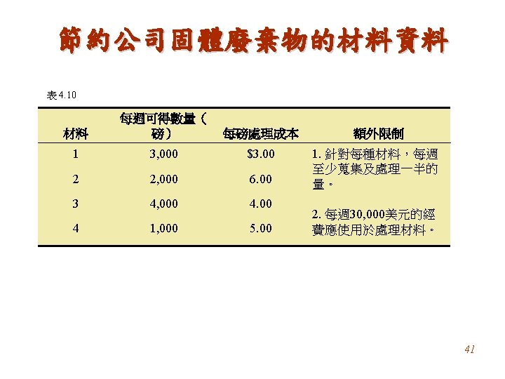
Example 4 -12 Agriculture Applications A farm owner in Des Moines, Iowa, is interested in determining how to divide the farmland among four different types of crops. The farmer owns two farms in separate locations and has decided to plant the following four types of crops in these farms: corn, wheat, bean, and cotton. The first farm consists of 1, 450 acres of land, while the second farm consists of 850 acres of land. Any of the four crops may be planted on either farm. However, after a survey of the land, based on the characteristics of the farmlands, Table 4 -7 shows the maximum acreage restrictions the farmer has placed for each crop. 94

95

96

97

98