INTRODUCTION TO LINEAR PROGRAMMING CONTENTS l Introduction to

INTRODUCTION TO LINEAR PROGRAMMING CONTENTS l Introduction to Linear Programming l Applications of Linear Programming Reference: Chapter 1 in BJS book. 1

Learning objectives u. Defining linear programs u. Understanding the main steps in modeling problems and assumptions of LPs u. Understanding modeling a problem through typical example problems u. Understanding the use of some modeling approaches u. Graphical approach to solve LPs u. Examining different types of LP wrt feasibility and boundedness 2

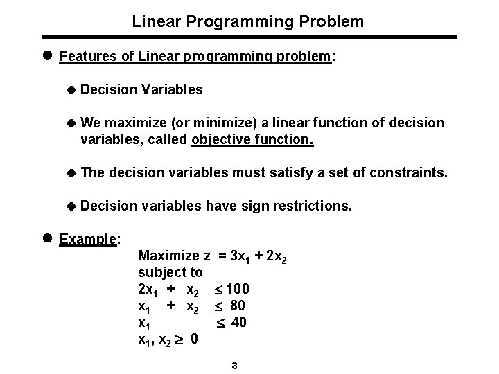
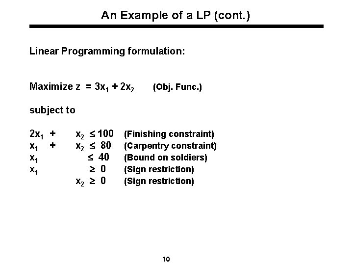
Linear Programming Problem l Features of Linear programming problem: u Decision Variables u We maximize (or minimize) a linear function of decision variables, called objective function. u The decision variables must satisfy a set of constraints. u Decision variables have sign restrictions. l Example: Maximize z subject to 2 x 1 + x 2 x 1 , x 2 0 = 3 x 1 + 2 x 2 100 80 40 3

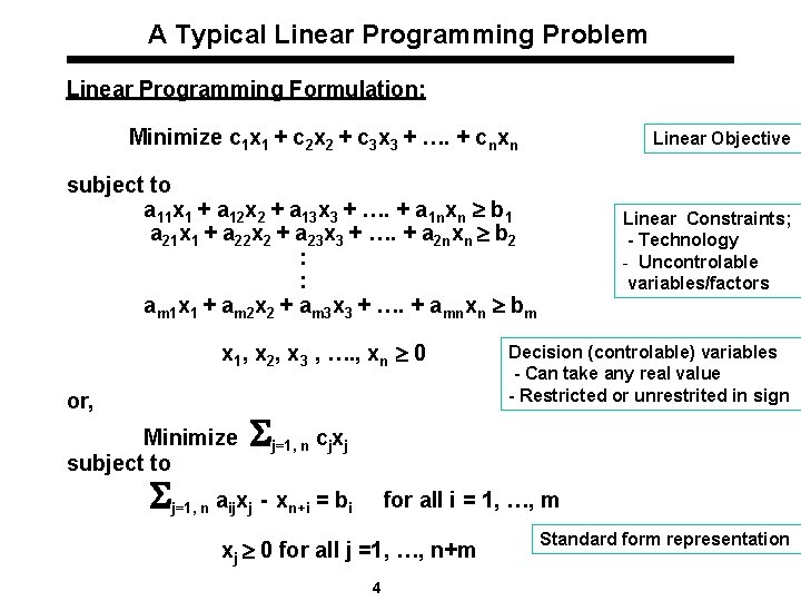
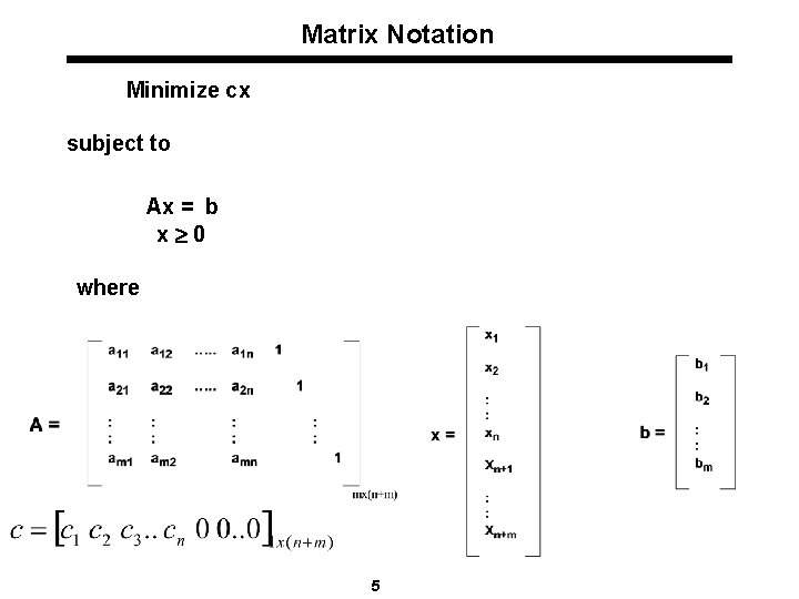
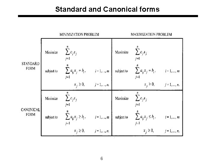
A Typical Linear Programming Problem Linear Programming Formulation: Minimize c 1 x 1 + c 2 x 2 + c 3 x 3 + …. + cnxn Linear Objective subject to a 11 x 1 + a 12 x 2 + a 13 x 3 + …. + a 1 nxn b 1 a 21 x 1 + a 22 x 2 + a 23 x 3 + …. + a 2 nxn b 2 : : am 1 x 1 + am 2 x 2 + am 3 x 3 + …. + amnxn bm x 1, x 2, x 3 , …. , xn 0 or, Minimize subject to Linear Constraints; - Technology - Uncontrolable variables/factors Decision (controlable) variables - Can take any real value - Restricted or unrestrited in sign j=1, n cjxj j=1, n aijxj - xn+i = bi for all i = 1, …, m xj 0 for all j =1, …, n+m 4 Standard form representation

Matrix Notation Minimize cx subject to Ax = b x 0 where 5

Standard and Canonical forms 6

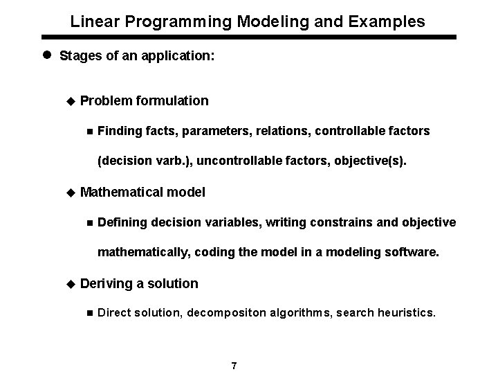
Linear Programming Modeling and Examples l Stages of an application: u Problem formulation n Finding facts, parameters, relations, controllable factors (decision varb. ), uncontrollable factors, objective(s). u Mathematical model n Defining decision variables, writing constrains and objective mathematically, coding the model in a modeling software. u Deriving a solution n Direct solution, decompositon algorithms, search heuristics. 7

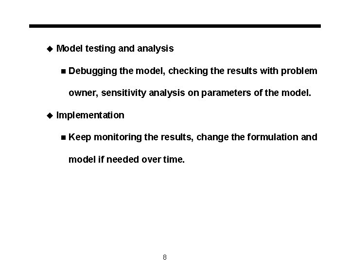
u Model testing and analysis n Debugging the model, checking the results with problem owner, sensitivity analysis on parameters of the model. u Implementation n Keep monitoring the results, change the formulation and model if needed over time. 8

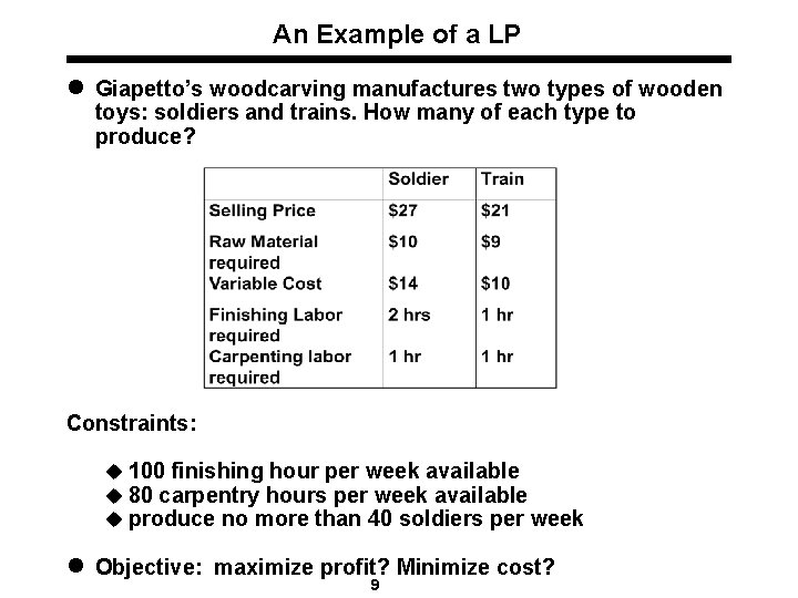
An Example of a LP l Giapetto’s woodcarving manufactures two types of wooden toys: soldiers and trains. How many of each type to produce? Constraints: u 100 finishing hour per week available u 80 carpentry hours per week available u produce no more than 40 soldiers per week l Objective: maximize profit? Minimize cost? 9

An Example of a LP (cont. ) Linear Programming formulation: Maximize z = 3 x 1 + 2 x 2 (Obj. Func. ) subject to 2 x 1 + x 1 x 2 100 x 2 80 40 0 x 2 0 (Finishing constraint) (Carpentry constraint) (Bound on soldiers) (Sign restriction) 10

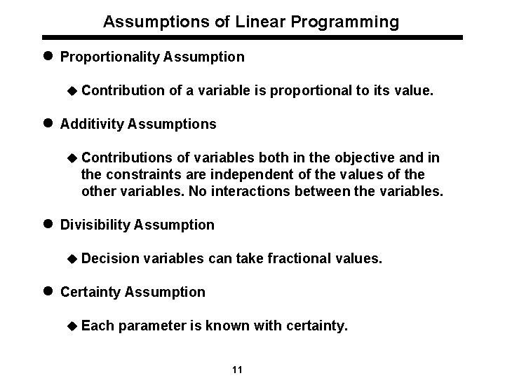
Assumptions of Linear Programming l Proportionality Assumption u Contribution of a variable is proportional to its value. l Additivity Assumptions u Contributions of variables both in the objective and in the constraints are independent of the values of the other variables. No interactions between the variables. l Divisibility Assumption u Decision variables can take fractional values. l Certainty Assumption u Each parameter is known with certainty. 11

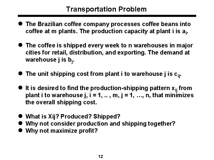
Transportation Problem l The Brazilian coffee company processes coffee beans into coffee at m plants. The production capacity at plant i is ai. l The coffee is shipped every week to n warehouses in major cities for retail, distribution, and exporting. The demand at warehouse j is bj. l The unit shipping cost from plant i to warehouse j is cij. l It is desired to find the production-shipping pattern xij from plant i to warehouse j, i = 1, . . , m, j = 1, …, n, that minimizes the overall shipping cost. l What is Xij? Produced? Shipped? l Why not consider production and shipping together? l Why not maximize profit? 12

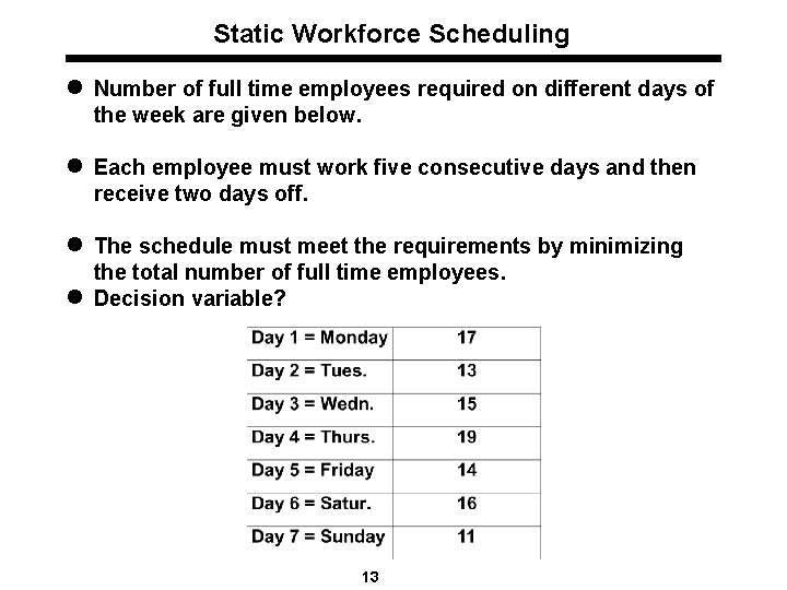
Static Workforce Scheduling l Number of full time employees required on different days of the week are given below. l Each employee must work five consecutive days and then receive two days off. l The schedule must meet the requirements by minimizing the total number of full time employees. l Decision variable? 13

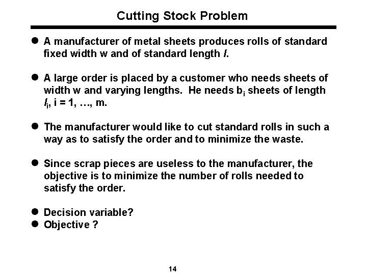
Cutting Stock Problem l A manufacturer of metal sheets produces rolls of standard fixed width w and of standard length l. l A large order is placed by a customer who needs sheets of width w and varying lengths. He needs bi sheets of length li, i = 1, …, m. l The manufacturer would like to cut standard rolls in such a way as to satisfy the order and to minimize the waste. l Since scrap pieces are useless to the manufacturer, the objective is to minimize the number of rolls needed to satisfy the order. l Decision variable? l Objective ? 14

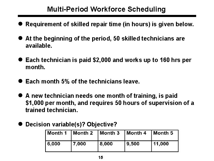
Multi-Period Workforce Scheduling l Requirement of skilled repair time (in hours) is given below. l At the beginning of the period, 50 skilled technicians are available. l Each technician is paid $2, 000 and works up to 160 hrs per month. l Each month 5% of the technicians leave. l A new technician needs one month of training, is paid $1, 000 per month, and requires 50 hours of supervision of a trained technician. l Decision variable(s)? Objective? 15

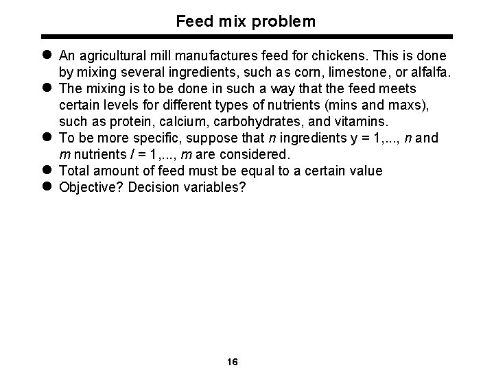
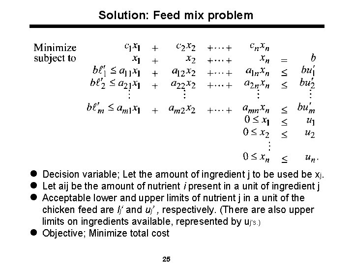
Feed mix problem l An agricultural mill manufactures feed for chickens. This is done l l by mixing several ingredients, such as corn, limestone, or alfalfa. The mixing is to be done in such a way that the feed meets certain levels for different types of nutrients (mins and maxs), such as protein, calcium, carbohydrates, and vitamins. To be more specific, suppose that n ingredients y = 1, . . . , n and m nutrients / = 1, . . . , m are considered. Total amount of feed must be equal to a certain value Objective? Decision variables? 16

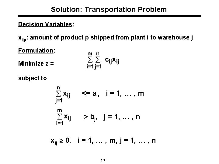
Solution: Transportation Problem Decision Variables: xijp: amount of product p shipped from plant i to warehouse j Formulation: Minimize z = subject to <= ai, i = 1, … , m bj, j = 1, … , n xij 0, i = 1, … , m, j = 1, … , n 17

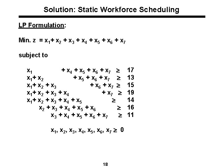
Solution: Static Workforce Scheduling LP Formulation: Min. z = x 1+ x 2 + x 3 + x 4 + x 5 + x 6 + x 7 subject to x 1 + x 4 + x 5 + x 6 + x 7 x 1 + x 2 + x 3 + x 4 + x 5 x 2 + x 3 + x 4 + x 5 + x 6 + x 7 x 1 , x 2 , x 3 , x 4 , x 5 , x 6 , x 7 0 18 17 13 15 19 14 16 11

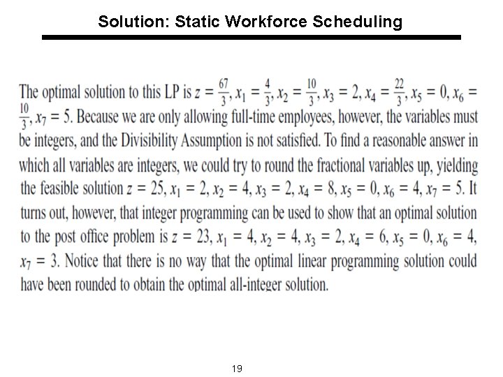
Solution: Static Workforce Scheduling 19

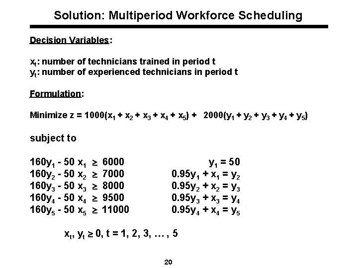
Solution: Multiperiod Workforce Scheduling Decision Variables: xt: number of technicians trained in period t yt: number of experienced technicians in period t Formulation: Minimize z = 1000(x 1 + x 2 + x 3 + x 4 + x 5) + 2000(y 1 + y 2 + y 3 + y 4 + y 5) subject to 160 y 1 - 50 x 1 160 y 2 - 50 x 2 160 y 3 - 50 x 3 160 y 4 - 50 x 4 160 y 5 - 50 x 5 6000 7000 8000 9500 11000 y 1 = 50 0. 95 y 1 + x 1 = y 2 0. 95 y 2 + x 2 = y 3 0. 95 y 3 + x 3 = y 4 0. 95 y 4 + x 4 = y 5 xt, yt 0, t = 1, 2, 3, … , 5 20

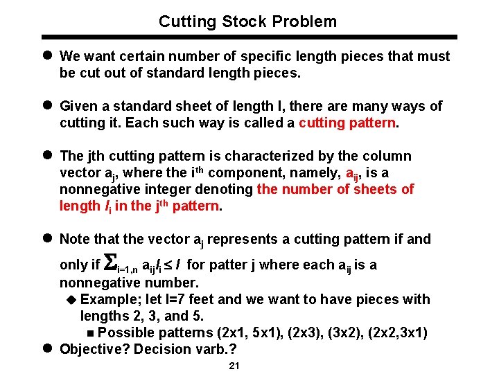
Cutting Stock Problem l We want certain number of specific length pieces that must be cut of standard length pieces. l Given a standard sheet of length l, there are many ways of cutting it. Each such way is called a cutting pattern. l The jth cutting pattern is characterized by the column vector aj, where the ith component, namely, aij, is a nonnegative integer denoting the number of sheets of length li in the jth pattern. l Note that the vector aj represents a cutting pattern if and only if i=1, n aijli l for patter j where each aij is a nonnegative number. u Example; let l=7 feet and we want to have pieces with lengths 2, 3, and 5. n Possible patterns (2 x 1, 5 x 1), (2 x 3), (3 x 2), (2 x 2, 3 x 1) l Objective? Decision varb. ? 21

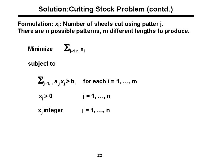
Solution: Cutting Stock Problem (contd. ) Formulation: xi: Number of sheets cut using patter j. There are n possible patterns, m different lengths to produce. Minimize j=1, n xi subject to j=1, n aij xj bi for each i = 1, …, m xj 0 j = 1, …, n xj integer j = 1, …, n 22

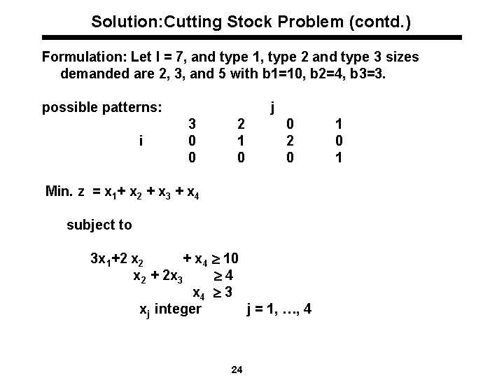
Solution: Cutting Stock Problem (contd. ) Formulation: Let l = 7, and type 1, type 2 and type 3 sizes demanded are 2, 3, and 5 with b 1=10, b 2=4, b 3=3. possible patterns: i j 3 0 0 2 1 0 0 2 0 Min. z = x 1+ x 2 + x 3 + x 4 subject to 3 x 1+2 x 2 + x 4 10 x 2 + 2 x 3 4 x 4 3 xj integer j = 1, …, 4 23 1 0 1

Solution: Cutting Stock Problem (contd. ) Formulation: Let l = 7, and type 1, type 2 and type 3 sizes demanded are 2, 3, and 5 with b 1=10, b 2=4, b 3=3. possible patterns: i j 3 0 0 2 1 0 0 2 0 Min. z = x 1+ x 2 + x 3 + x 4 subject to 3 x 1+2 x 2 + x 4 10 x 2 + 2 x 3 4 x 4 3 xj integer j = 1, …, 4 24 1 0 1

Solution: Feed mix problem l Decision variable; Let the amount of ingredient j to be used be xj. l Let aij be the amount of nutrient i present in a unit of ingredient j l Acceptable lower and upper limits of nutrient j in a unit of the chicken feed are lj‘ and uj’ , respectively. (There also upper limits on ingredients available, represented by uj’s. ) l Objective; Minimize total cost 25

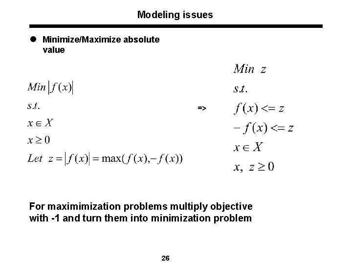
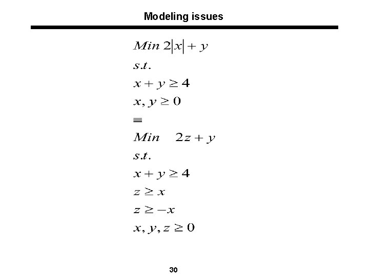
Modeling issues l Minimize/Maximize absolute value => For maximimization problems multiply objective with -1 and turn them into minimization problem 26

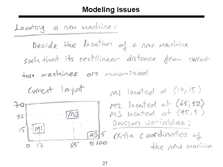
Modeling issues 27

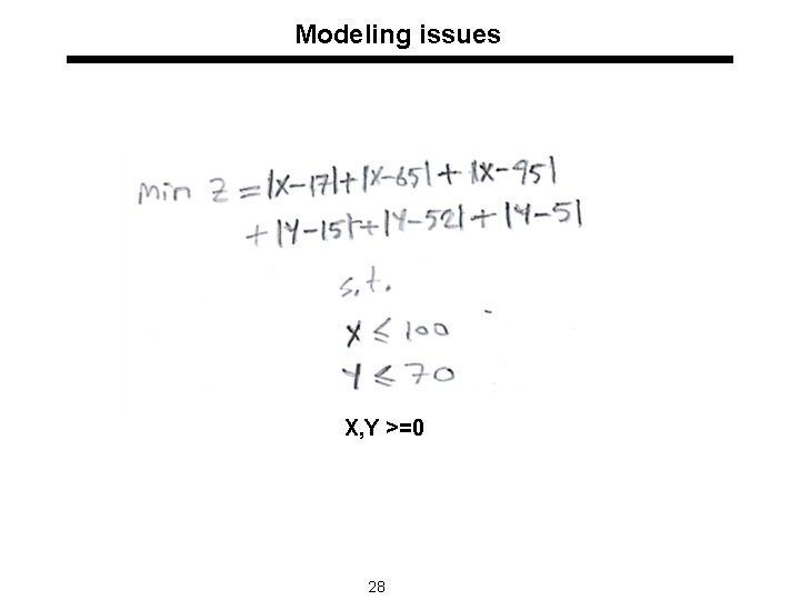
Modeling issues X, Y >=0 28

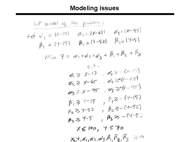
Modeling issues 29

Modeling issues 30

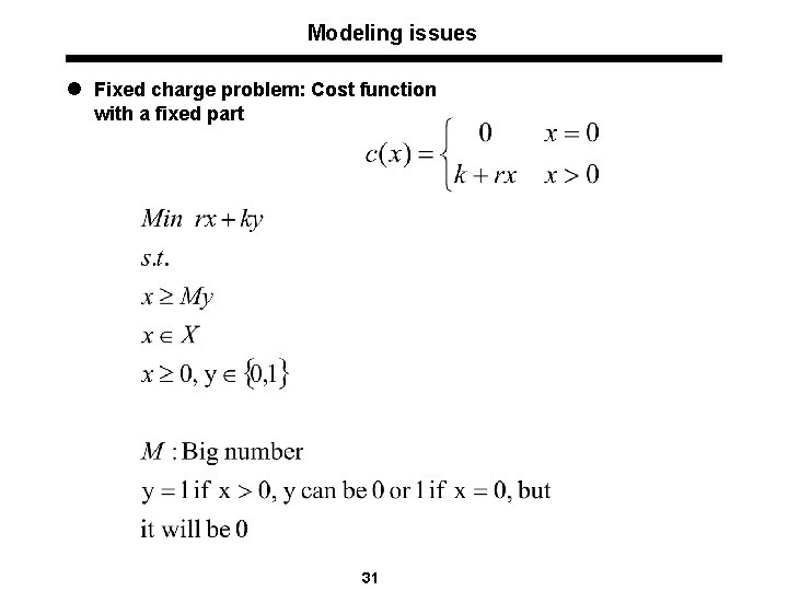
Modeling issues l Fixed charge problem: Cost function with a fixed part 31

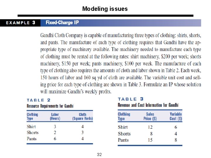
Modeling issues 32

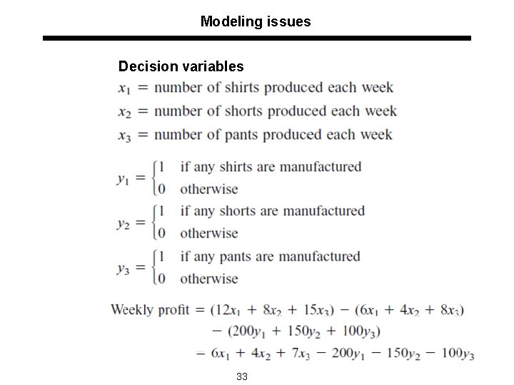
Modeling issues Decision variables 33

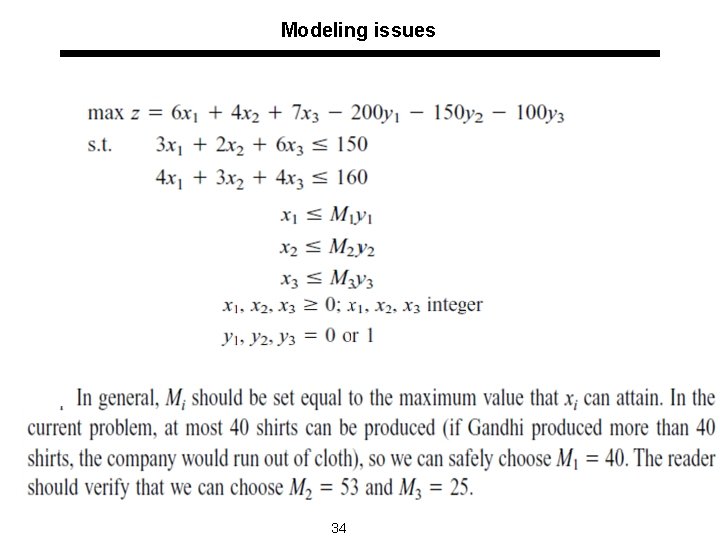
Modeling issues 34

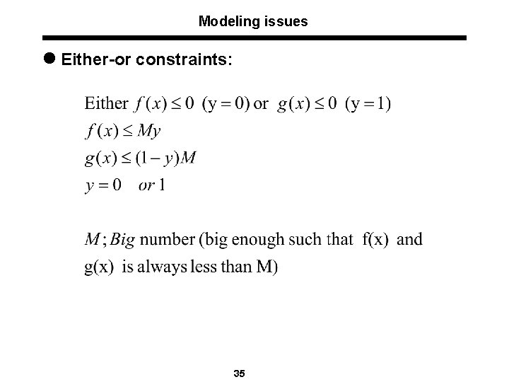
Modeling issues l Either-or constraints: 35

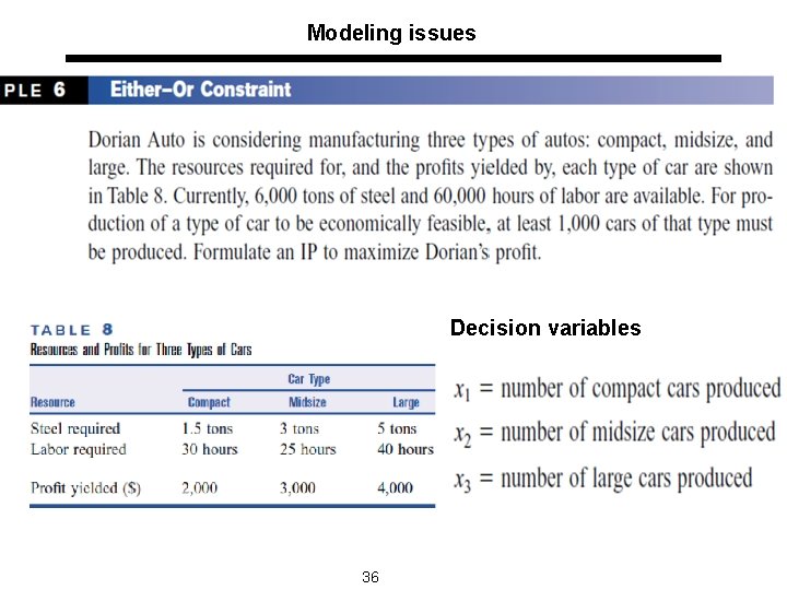
Modeling issues Decision variables 36

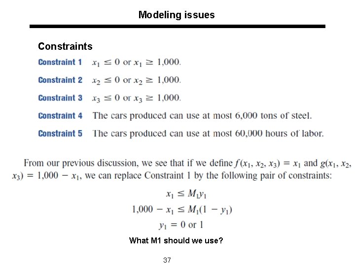
Modeling issues Constraints What M 1 should we use? 37

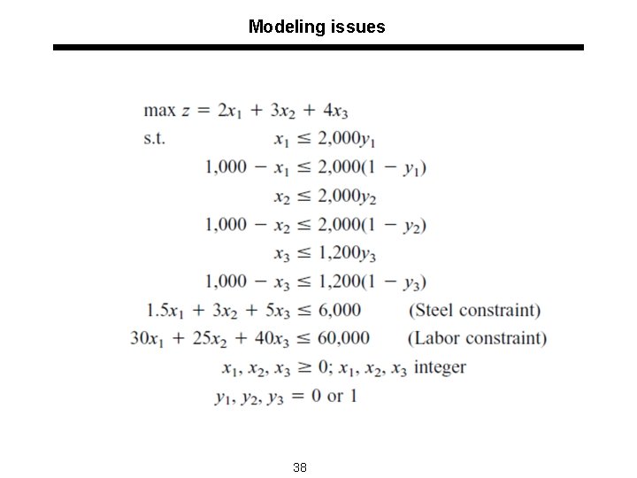
Modeling issues 38

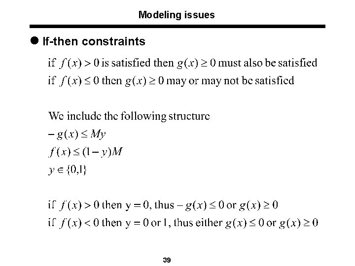
Modeling issues l If-then constraints 39

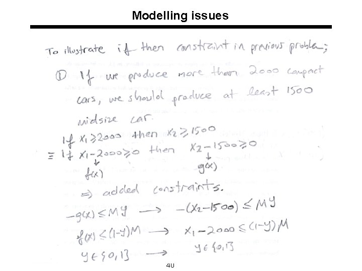
Modelling issues 40

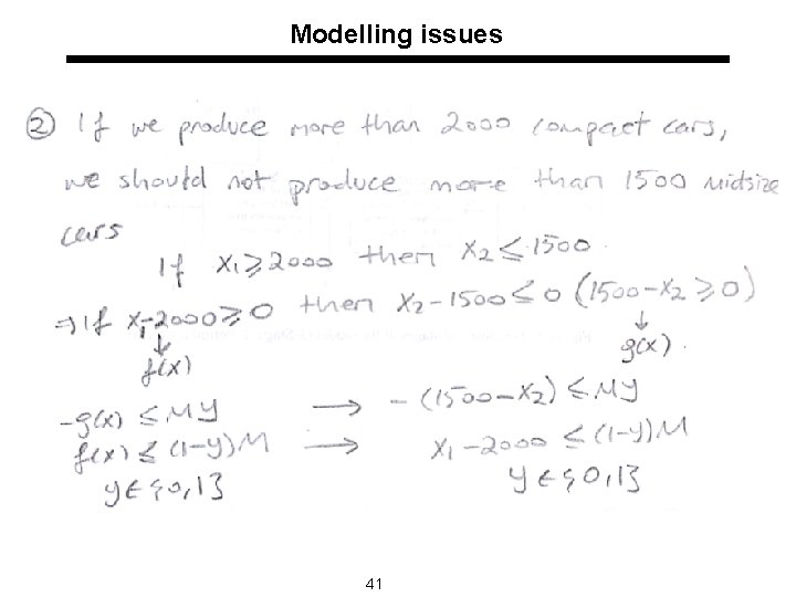
Modelling issues 41

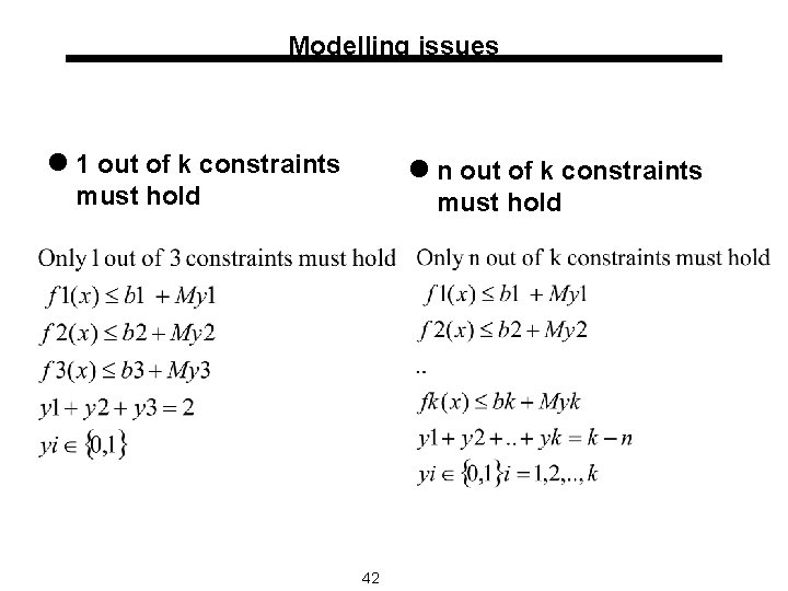
Modelling issues l 1 out of k constraints l n out of k constraints must hold 42

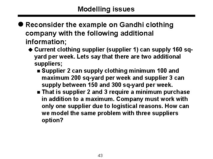
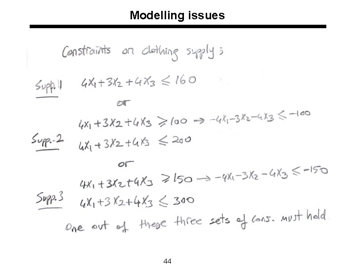
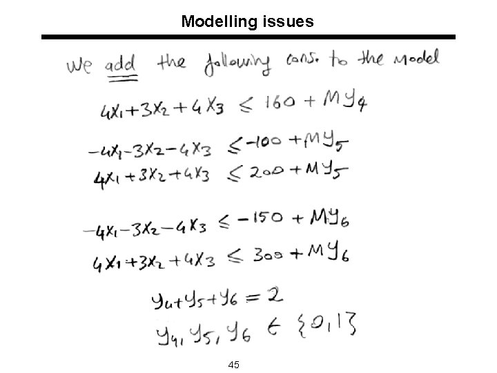
Modelling issues l Reconsider the example on Gandhi clothing company with the following additional information; u Current clothing supplier (supplier 1) can supply 160 sq- yard per week. Lets say that there are two additional suppliers; n Supplier 2 can supply clothing minimum 100 and maximum 200 sq-yard per week and supplier 3 can supply between 150 and 300 sq-yard per week. n That is supplier 2 and 3 require a minimum purchase in addition to a maximum. Company must work with only one supplier due to logistical reasons. How can we model the same problem with three suppliers option? 43

Modelling issues 44

Modelling issues 45

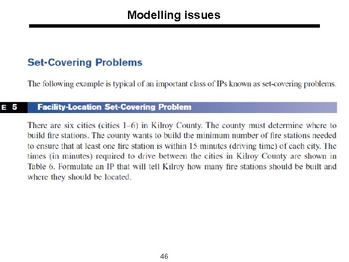
Modelling issues 46

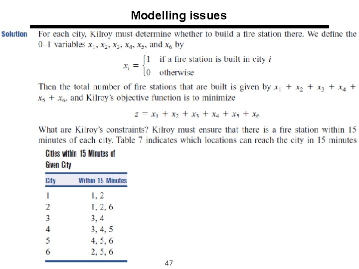
Modelling issues 47

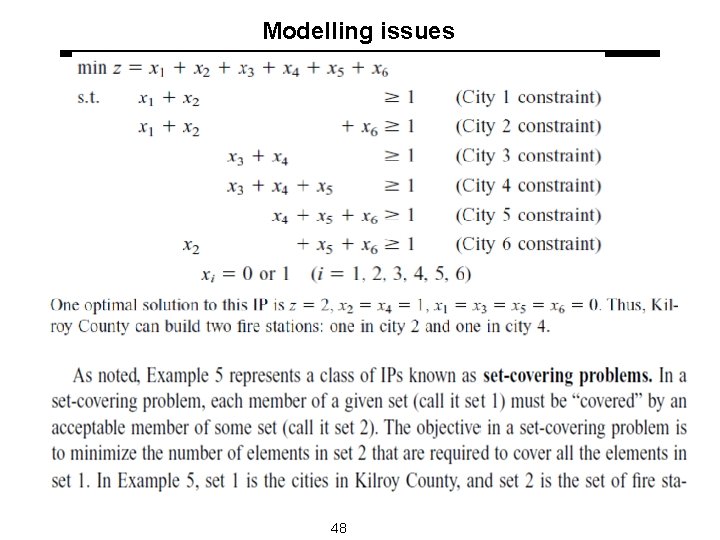
Modelling issues 48

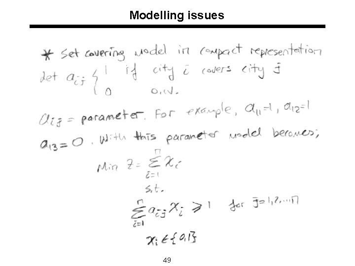
Modelling issues 49

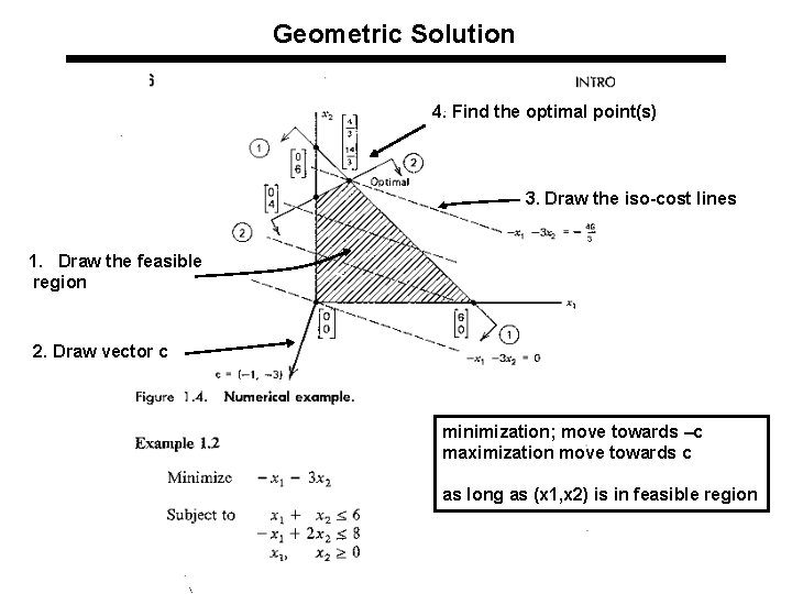
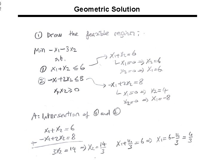
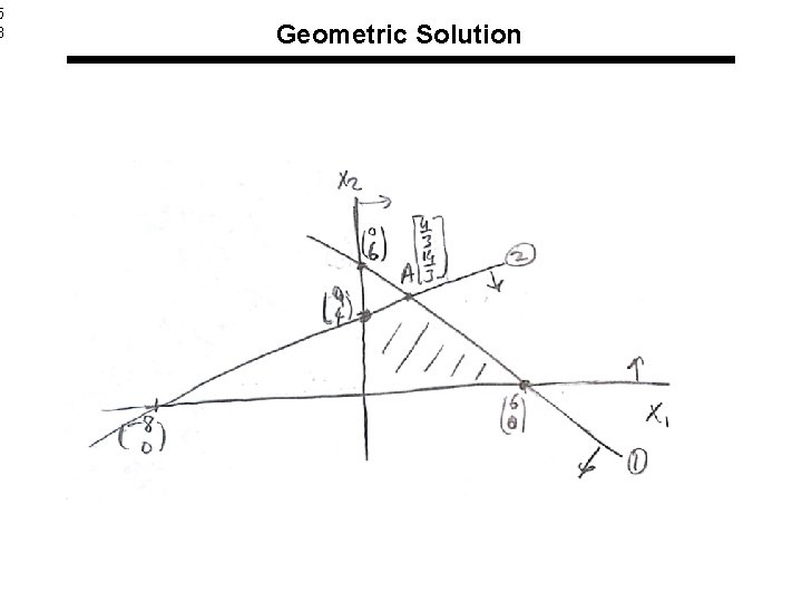
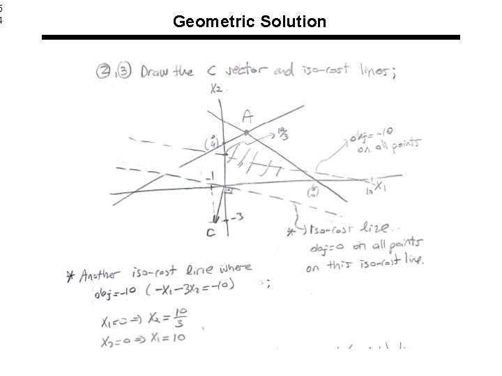
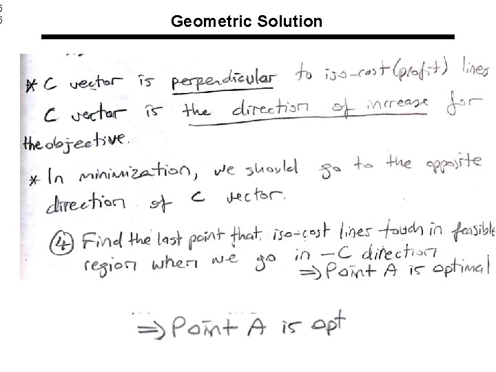
Geometric Solution l. Steps of the geometric solution 1. Determine and draw the feasible region 2. Draw the c vector 3. Draw the iso cost lines (perpendicular to c vector) 4. Find the last point(s) that iso-cost lines touch the feasible region, when we move towards direction of –c (in minimization). This point (or points) is the optimal solution.

Geometric Solution 4. Find the optimal point(s) 3. Draw the iso-cost lines 1. Draw the feasible region 2. Draw vector c minimization; move towards –c maximization move towards c as long as (x 1, x 2) is in feasible region

5 2 Geometric Solution

5 3 Geometric Solution

5 4 Geometric Solution

5 5 Geometric Solution

5 6 Unique finite optimal solution

5 7 Alternative finite optimal solution

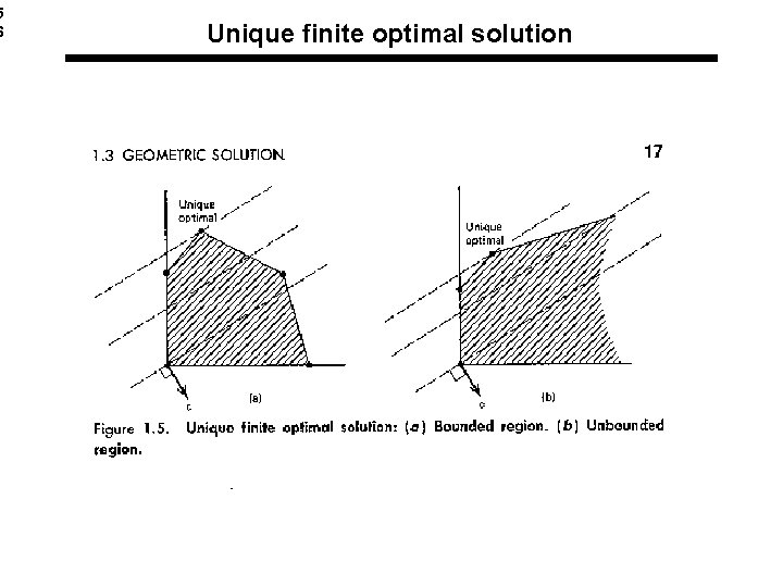
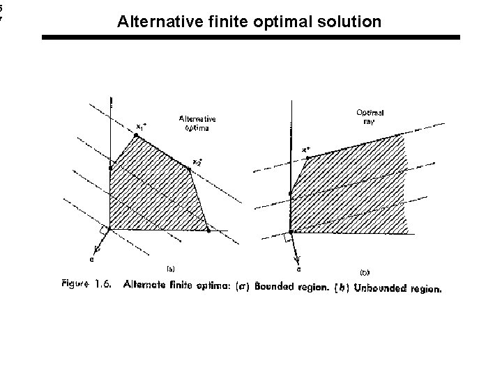
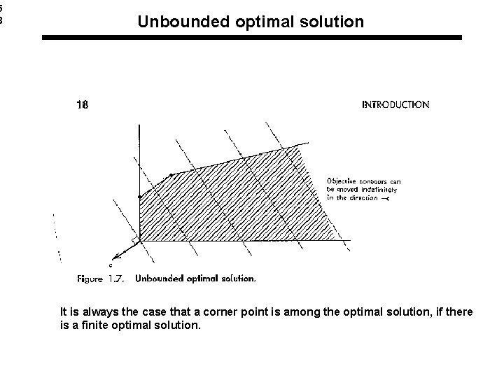
5 8 Unbounded optimal solution It is always the case that a corner point is among the optimal solution, if there is a finite optimal solution.

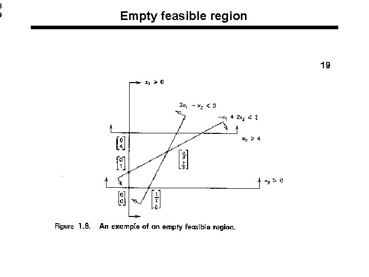
5 9 Empty feasible region