Introduction to Linear and Nonlinear Programming 1 Outline

Introduction to Linear and Nonlinear Programming 1

Outline § Introduction - types of problems - size of problems - iterative algorithms and convergence § Basic properties of Linear Programs - introduction - examples of linear programming problems 2

Types of Problems Three parts - linear programming - unconstrained problems - constrained problems § The last two parts comprise the subject of nonlinear programming § 3

Linear Programming 1. It is characterized by linear functions of the unknowns; the objective is linear in the unknowns, and the constraints are linear equalities or linear inequalities. 1. Why are linear forms for objectives and constraints so popular in problem formulation? - a great number of constraints and objectives that arise in practice are indisputably linear (ex: budget constraint) - they are often the least difficult to define 4

Unconstrained Problems § Are unconstrained problems devoid of structural properties as to preclude their applicability as useful models of meaningful problems? - if the scope of a problem is broadened to the consideration of all relevant decision variables, there may then be no constraints - many constrained problems are sometimes easily converted to unconstrained problems 5

Constrained Problems § Many complex problems cannot be directly treated in its entirety accounting for all possible choices, but instead must be decomposed into separate subproblems § “Continuous variable programming” 6

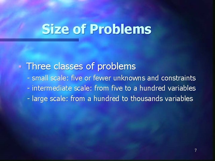
Size of Problems § Three classes of problems - small scale: five or fewer unknowns and constraints - intermediate scale: from five to a hundred variables - large scale: from a hundred to thousands variables 7

Iterative Algorithms and Convergence Most algorithms designed to solve large optimization problems are iterative. § For LP problems, the generated sequence is of finite length, reaching the solution point exactly after a finite number of steps. § For non-LP problems, the sequence generally does not ever exactly reach the solution point, but converges toward it. § 8

Iterative Algorithms and Convergence (cont’d) § Iterative algorithms 1. the creation of the algorithms themselves 2. the verification that a given algorithm will in fact generate a sequence that converges to a solution 3. the rate at which the generated sequence of points converges to the solution § Convergence rate theory 1. theory is, for the most part, extremely simple in nature 2. a large class of seemingly distinct algorithms turns out to have a common convergence rate 9

LP Problems’ Standard Form 10

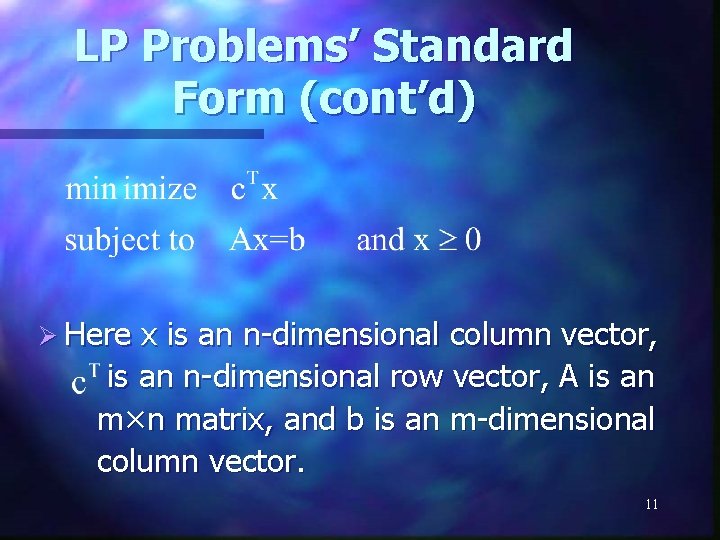
LP Problems’ Standard Form (cont’d) Ø Here x is an n-dimensional column vector, is an n-dimensional row vector, A is an m×n matrix, and b is an m-dimensional column vector. 11

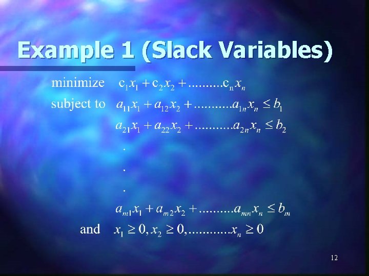
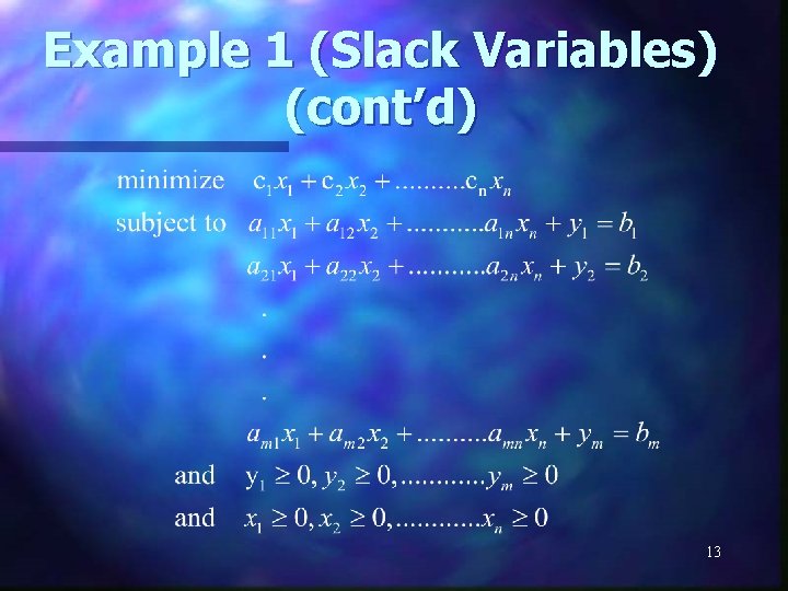
Example 1 (Slack Variables) 12

Example 1 (Slack Variables) (cont’d) 13

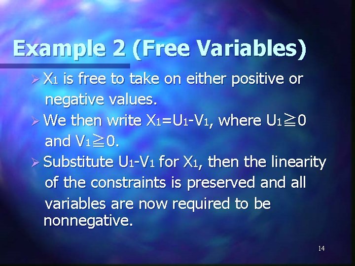
Example 2 (Free Variables) Ø X 1 is free to take on either positive or negative values. Ø We then write X 1=U 1 -V 1, where U 1≧ 0 and V 1≧ 0. Ø Substitute U 1 -V 1 for X 1, then the linearity of the constraints is preserved and all variables are now required to be nonnegative. 14

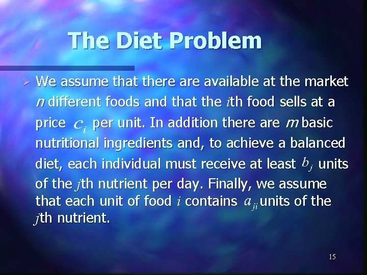
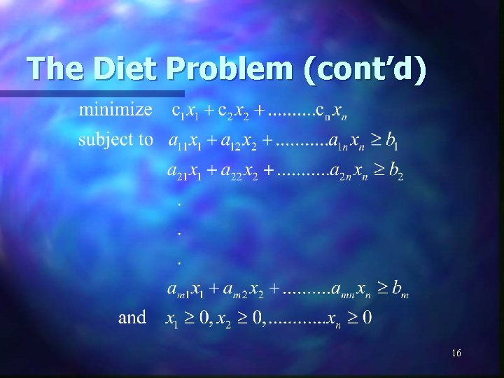
The Diet Problem Ø We assume that there available at the market n different foods and that the ith food sells at a price per unit. In addition there are m basic nutritional ingredients and, to achieve a balanced diet, each individual must receive at least units of the jth nutrient per day. Finally, we assume that each unit of food i contains units of the jth nutrient. 15

The Diet Problem (cont’d) 16

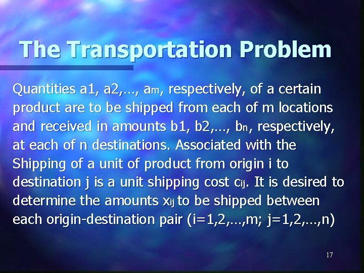
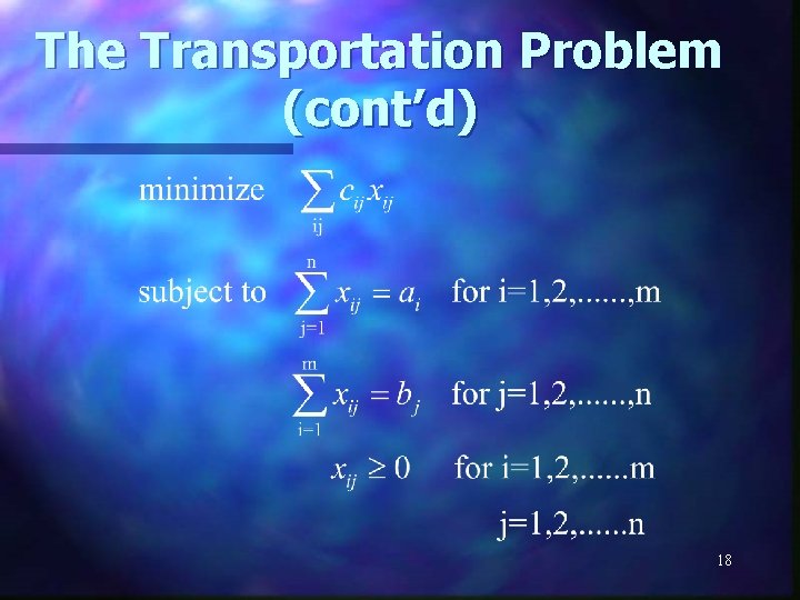
The Transportation Problem Quantities a 1, a 2, …, am, respectively, of a certain product are to be shipped from each of m locations and received in amounts b 1, b 2, …, bn, respectively, at each of n destinations. Associated with the Shipping of a unit of product from origin i to destination j is a unit shipping cost cij. It is desired to determine the amounts xij to be shipped between each origin-destination pair (i=1, 2, …, m; j=1, 2, …, n) 17

The Transportation Problem (cont’d) 18