Introduction to Klampt Kris Hauser ECE 383 ME

Introduction to Klamp’t Kris Hauser ECE 383 / ME 442

Agenda • Intro to Klamp’t • Key concepts • • • World Robot Configuration Link IK Objective IK Solver • Klamp’t Python API

What is Klamp’t? • A suite of software tools for planning and simulation of many-DOF robots • Planning: state-of-the-art • Simulation: state-of-the-art • Feedback control: some basic functionality • System integration: some tools for linking with ROS • Perception: nothing whatsoever • Intended audiences: primarily education & research • Cross platform: Linux, Mac, Windows • Languages: C++ and Python • Team • Lead: Kris Hauser • Contributors: Jordan Tritell, Jingru Luo, Alessio Rocchi • Mac build: Adam Konnecker, Cam Allen, Steve Kuznetsov

Historical context • Comparable packages: • Open. RAVE: probably most similar, not much legged robot support, simulation not as stable • ROS: is primarily a system integration tool, very steep learning curve esp. for non-CS types • With KDL/Move. It!/Gazebo packages, can have similar functionality to Klamp’t • Robot simulators, e. g. , V-REP, Webots, Gazebo: have more tools for behavior scripting, fewer tools for planning / analysis, simulation less stable • Klamp’t was developed from a historical code base (c. 2007), integrated with simulation in 2009, first release in 2014 • Started about the same time as Open. RAVE • To collect and reuse research products (and byproducts) • During DARPA Robotics Challenge, simulation was found much more stable than the dominant robot simulator, Gazebo, leading to first release

Design philosophy • Give students/researchers/engineers convenient programming tools for: • Learning robotics • Analyzing robots • Prototyping & developing intelligent robot behaviors • Once behaviors are developed in simulation, a user can apply them to their robot using ROS… or DIY system integration

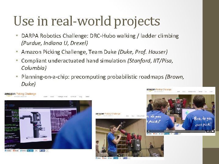
Use in real-world projects • DARPA Robotics Challenge: DRC-Hubo walking / ladder climbing (Purdue, Indiana U, Drexel) • Amazon Picking Challenge, Team Duke (Duke, Prof. Hauser) • Compliant underactuated hand simulation (Stanford, IIT/Pisa, Columbia) • Planning-on-a-chip: precomputing probabilistic roadmaps (Brown, Duke)

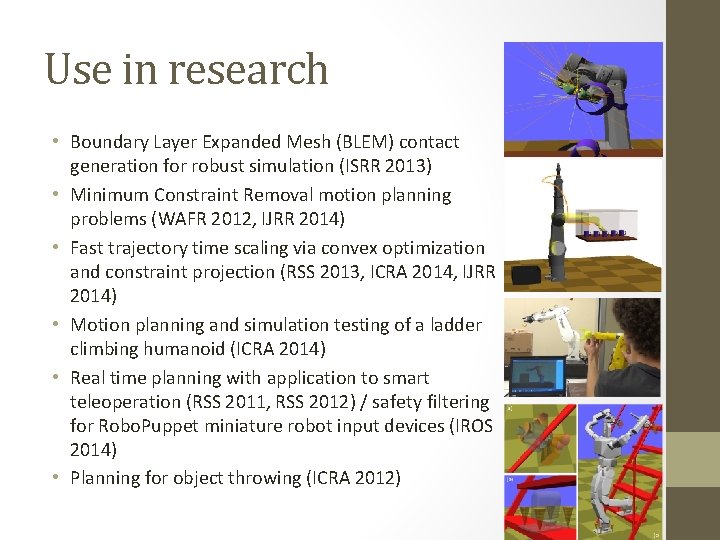
Use in research • Boundary Layer Expanded Mesh (BLEM) contact generation for robust simulation (ISRR 2013) • Minimum Constraint Removal motion planning problems (WAFR 2012, IJRR 2014) • Fast trajectory time scaling via convex optimization and constraint projection (RSS 2013, ICRA 2014, IJRR 2014) • Motion planning and simulation testing of a ladder climbing humanoid (ICRA 2014) • Real time planning with application to smart teleoperation (RSS 2011, RSS 2012) / safety filtering for Robo. Puppet miniature robot input devices (IROS 2014) • Planning for object throwing (ICRA 2012)

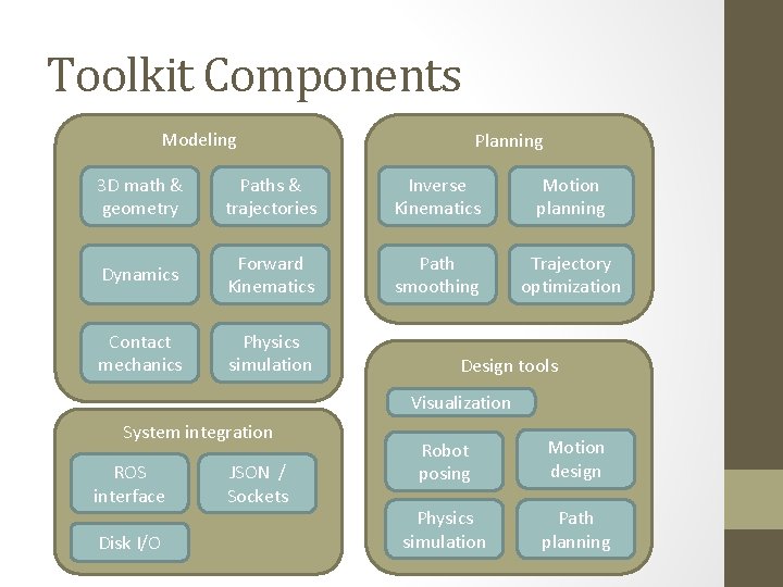
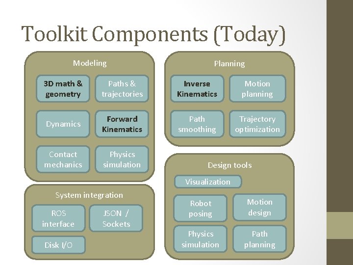
Toolkit Components Modeling Planning 3 D math & geometry Paths & trajectories Inverse Kinematics Motion planning Dynamics Forward Kinematics Path smoothing Trajectory optimization Contact mechanics Physics simulation Design tools Visualization System integration ROS interface Disk I/O JSON / Sockets Robot posing Motion design Physics simulation Path planning

Toolkit Components (Today) Modeling Planning 3 D math & geometry Paths & trajectories Inverse Kinematics Motion planning Dynamics Forward Kinematics Path smoothing Trajectory optimization Contact mechanics Physics simulation Design tools Visualization System integration ROS interface Disk I/O JSON / Sockets Robot posing Motion design Physics simulation Path planning

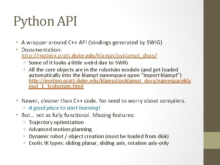
Python API • A wrapper around C++ API (bindings generated by SWIG) • Documentation: http: //motion. pratt. duke. edu/klampt/pyklampt_docs/ • Some of it looks a little weird due to SWIG • All the core objects are in the robotsim module (and get loaded automatically into the klampt namespace upon “import klampt”) http: //motion. pratt. duke. edu/klampt/pyklampt_docs/namespacekla mpt_1_1 robotsim. html • Newer, cleaner than C++ code. No need to worry about compilers. • A good place to start learning! • But… not as fully functional. Missing features: • Trajectory optimization • Advanced motion planning • Dynamic robot / object creation (must be loaded from disk) • Exotic IK types: sliding planar, sliding axis, rotation axis-only

Assumptions • You have read / understood the Klamp’t Python math tutorial http: //motion. pratt. duke. edu/klampt/tutorial_math. html

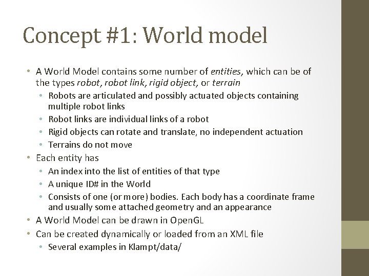
Concept #1: World model • A World Model contains some number of entities, which can be of the types robot, robot link, rigid object, or terrain • Robots are articulated and possibly actuated objects containing multiple robot links • Robot links are individual links of a robot • Rigid objects can rotate and translate, no independent actuation • Terrains do not move • Each entity has • An index into the list of entities of that type • A unique ID# in the World • Consists of one (or more) bodies. Each body has a coordinate frame and usually some attached geometry and an appearance • A World Model can be drawn in Open. GL • Can be created dynamically or loaded from an XML file • Several examples in Klampt/data/

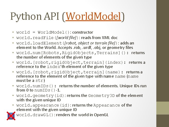
Python API (World. Model) • world = World. Model(): constructor • world. read. File([world file]): reads from XML doc • world. load. Element([robot, object or terrain file]): adds an element to the World. Accepts. rob, . urdf, . obj, or geometry files • world. num[Robots, Rigid. Objects, Terrains](): returns the number of elements of the given type • world. [robot, rigid. Object, terrain](index): returns a reference to the index’th element of the given type • world. [robot, rigid. Object, terrain](name): returns a reference to the element of the given type with name (name must be a str) • world. num. IDs(): returns the number of elements. Unique IDs run from 0 to num. IDs()-1. • world. geometry(id): returns the Geometry 3 D of the element with the given unique ID • world. appearance(id): returns the Appearance of the element with the given unique ID • world. draw. GL(): renders the world in Open. GL

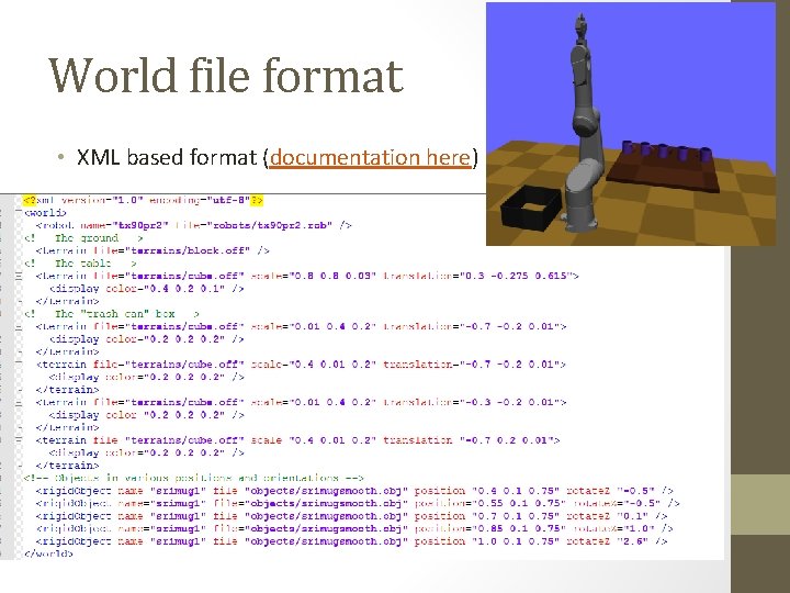
World file format • XML based format (documentation here)

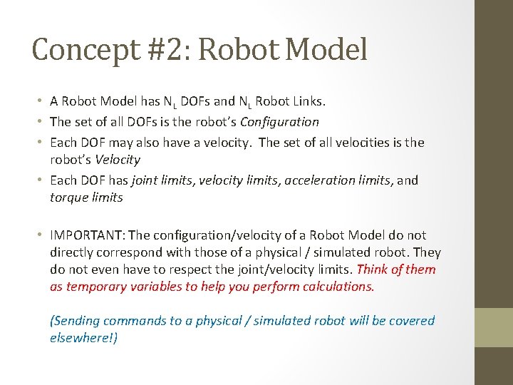
Concept #2: Robot Model • A Robot Model has NL DOFs and NL Robot Links. • The set of all DOFs is the robot’s Configuration • Each DOF may also have a velocity. The set of all velocities is the robot’s Velocity • Each DOF has joint limits, velocity limits, acceleration limits, and torque limits • IMPORTANT: The configuration/velocity of a Robot Model do not directly correspond with those of a physical / simulated robot. They do not even have to respect the joint/velocity limits. Think of them as temporary variables to help you perform calculations. (Sending commands to a physical / simulated robot will be covered elsewhere!)

Python API (Robot. Model) • robot = world. robot([name or index]): access Robot model reference • robot. get. ID(): gets the unique ID of the Robot model in the World model • robot. num[Links/Drivers](): returns the number of links or drivers (joints are abstracted away in the Python API) • robot. [link/driver](index): returns a reference to the index’th Robot. Model. Link / Robot. Model. Driver • robot. [link/driver](name): returns a reference to the Robot. Model. Link / Robot. Model. Driver with the given name (name must have type str) • robot. get[Config/Velocity](): returns the model’s Configuration/Velocity as a list of floats with length num. Links() • robot. set. Config(q): sets the model’s Configuration to q given as a list/tuple of floats with length num. Links(). Also, updates the forward kinematics of all Robot Links. • robot. set. Velocity(dq): sets the model’s Velocity to dq given as a list/tuple of floats with length num. Links() • robot. get[Joint/Velocity/Acceleration]Limits(): returns minimum/maximum of model’s Configuration/Velocity/acceleration as a pair of lists of floats with length num. Links() • robot. set[Joint/Velocity/Acceleration]Limits(vmin, vmax): sets minimum/maximum Configuration/Velocity/acceleration given two lists of floats with length num. Links() • robot. draw. GL(): renders the robot in Open. GL

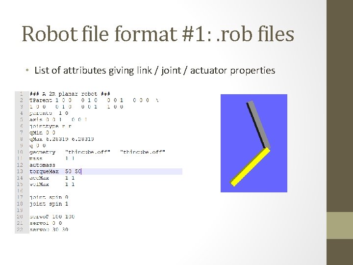
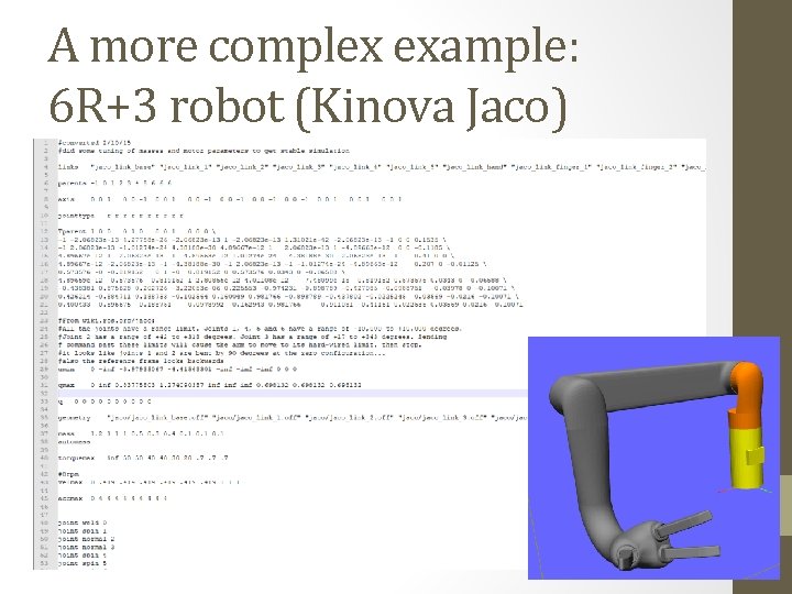
Robot file format #1: . rob files • List of attributes giving link / joint / actuator properties

A more complex example: 6 R+3 robot (Kinova Jaco)

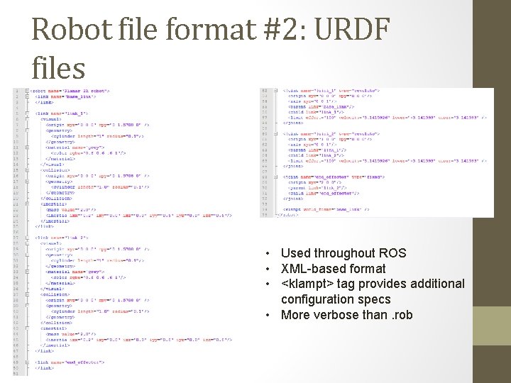
Robot file format #2: URDF files • Used throughout ROS • XML-based format • <klampt> tag provides additional configuration specs • More verbose than. rob

Concept #3: Robot link model • A Robot Link corresponds to one of the robot model’s DOFs • It holds all information about the link in its reference coordinate frame (name, index, parent, reference transform to parent, type of joint, joint axis, mass) • It also holds information regarding its current transform given the robot model’s current configuration (calculated via forward kinematics) • It also helps you calculate Jacobians, velocities, etc

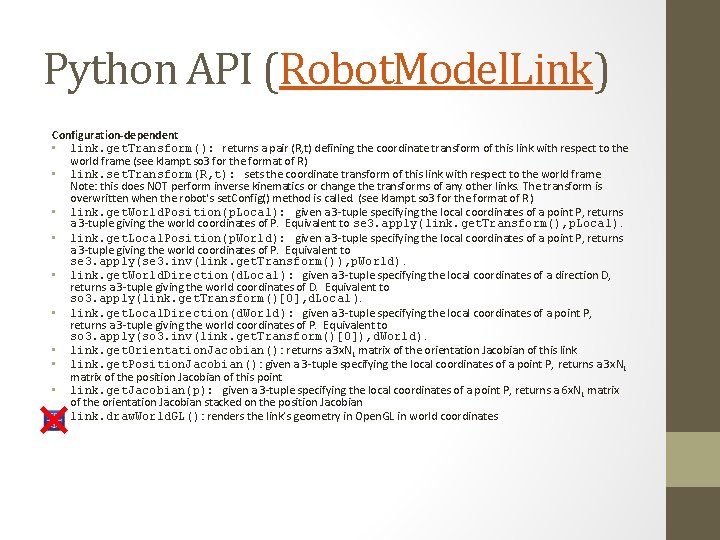
Python API (Robot. Model. Link) Configuration-independent • link = robot. link([name or index]): access Robot Link reference • link. get. ID(): gets the unique ID of the Robot Link in the World model • link. get. Name(): returns a string naming this link • link. get. Robot(): returns a Robot. Model to which this link belongs • link. get. Index(): returns the link index on the Robot. Model for this link • link. get. Parent(): returns the index of the link’s parent (-1 for no parent) • link. set. Parent(p): sets the index of the link’s parent (-1 for no parent) • link. get. Axis(): returns a 3 -tuple of the link’s rotation/translation axis in local coordinates • link. set. Axis(axis): sets the link’s rotation/translation axis to the given 3 -tuple, specifying its local coordinates • link. get. Parent. Transform(): returns a pair (R, t) defining the reference coordinate transform of this link with respect to its parent (see klampt. so 3 for the format of R) • link. set. Parent. Transform(R, t): sets the reference coordinate transform of this link with respect to its parent (see klampt. so 3 for the format of R) • link. geometry(): returns a reference to the Geometry 3 D attached to this link • link. appearance(): returns a reference to the Appearance attached to this link • link. get. Mass(): returns the link’s Mass structure • link. set. Mass(mass): sets the link’s Mass structure • link. draw. Local. GL(): renders the link’s geometry in Open. GL in local coordinates

Python API (Robot. Model. Link) Configuration-dependent • link. get. Transform(): returns a pair (R, t) defining the coordinate transform of this link with respect to the world frame (see klampt. so 3 for the format of R) • link. set. Transform(R, t): sets the coordinate transform of this link with respect to the world frame. Note: this does NOT perform inverse kinematics or change the transforms of any other links. The transform is overwritten when the robot's set. Config() method is called. (see klampt. so 3 for the format of R) • link. get. World. Position(p. Local): given a 3 -tuple specifying the local coordinates of a point P, returns a 3 -tuple giving the world coordinates of P. Equivalent to se 3. apply(link. get. Transform(), p. Local). • link. get. Local. Position(p. World): given a 3 -tuple specifying the local coordinates of a point P, returns a 3 -tuple giving the world coordinates of P. Equivalent to se 3. apply(se 3. inv(link. get. Transform()), p. World). • link. get. World. Direction(d. Local ): given a 3 -tuple specifying the local coordinates of a direction D, returns a 3 -tuple giving the world coordinates of D. Equivalent to so 3. apply(link. get. Transform()[0], d. Local ). • link. get. Local. Direction(d. World ): given a 3 -tuple specifying the local coordinates of a point P, returns a 3 -tuple giving the world coordinates of P. Equivalent to so 3. apply(so 3. inv(link. get. Transform()[0]), d. World). • link. get. Orientation. Jacobian() : returns a 3 x. NL matrix of the orientation Jacobian of this link • link. get. Position. Jacobian (): given a 3 -tuple specifying the local coordinates of a point P, returns a 3 x. NL matrix of the position Jacobian of this point • link. get. Jacobian(p): given a 3 -tuple specifying the local coordinates of a point P, returns a 6 x. NL matrix of the orientation Jacobian stacked on the position Jacobian • link. draw. World. GL(): renders the link’s geometry in Open. GL in world coordinates

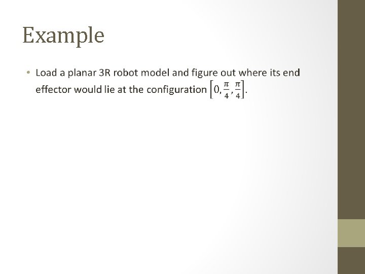
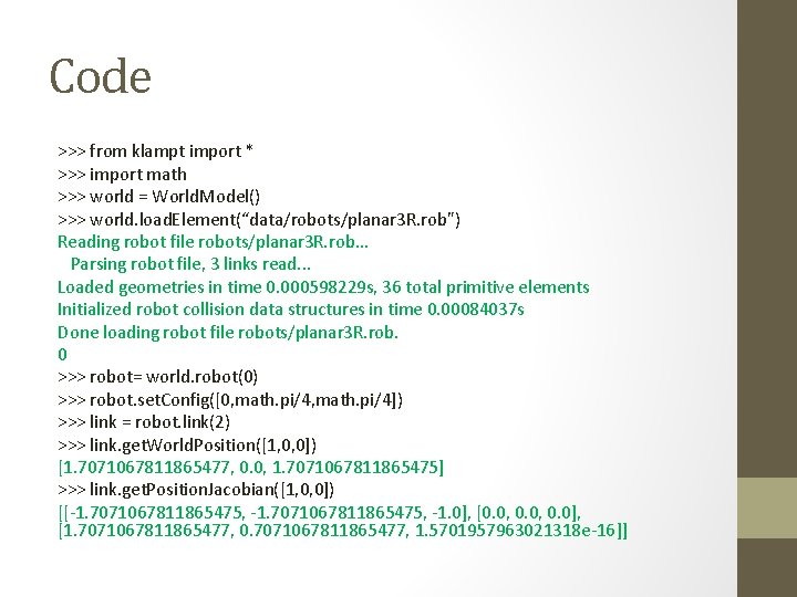
Example •

Code >>> from klampt import * >>> import math >>> world = World. Model() >>> world. load. Element(“data/robots/planar 3 R. rob") Reading robot file robots/planar 3 R. rob. . . Parsing robot file, 3 links read. . . Loaded geometries in time 0. 000598229 s, 36 total primitive elements Initialized robot collision data structures in time 0. 00084037 s Done loading robot file robots/planar 3 R. rob. 0 >>> robot= world. robot(0) >>> robot. set. Config([0, math. pi/4]) >>> link = robot. link(2) >>> link. get. World. Position([1, 0, 0]) [1. 7071067811865477, 0. 0, 1. 7071067811865475] >>> link. get. Position. Jacobian([1, 0, 0]) [[-1. 7071067811865475, -1. 0], [0. 0, 0. 0], [1. 7071067811865477, 0. 7071067811865477, 1. 5701957963021318 e-16]]

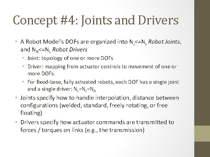
Concept #4: Joints and Drivers • A Robot Model’s DOFs are organized into NJ<=NL Robot Joints, and ND<=NL Robot Drivers • Joint: topology of one or more DOFs • Driver: mapping from actuator controls to movement of one or more DOFs. • For fixed-base, fully actuated robots, each DOF has a single joint and a single driver: NL=NJ=ND • Joints specify how to handle interpolation, distance between configurations (welded, standard, freely rotating, or free floating) • Drivers specify how actuator commands are transmitted to forces / torques on links (e. g. , the transmission)

Example

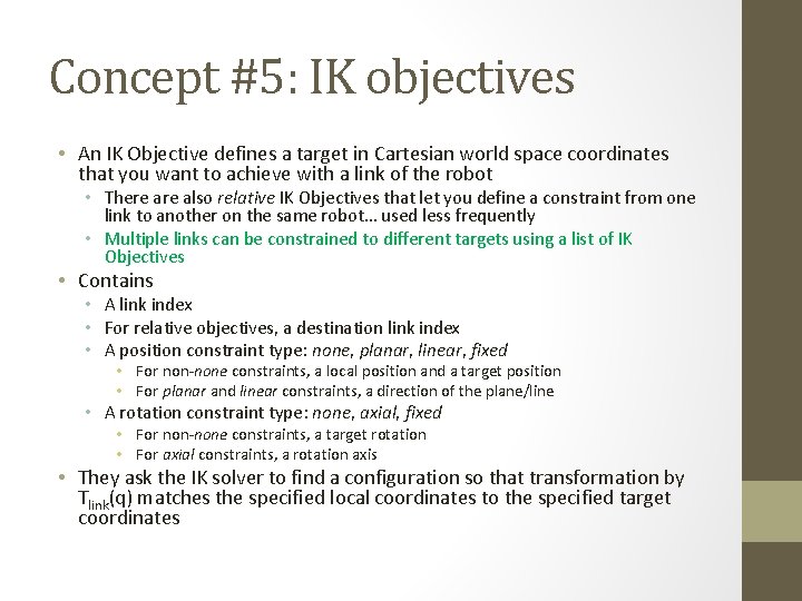
Concept #5: IK objectives • An IK Objective defines a target in Cartesian world space coordinates that you want to achieve with a link of the robot • There also relative IK Objectives that let you define a constraint from one link to another on the same robot… used less frequently • Multiple links can be constrained to different targets using a list of IK Objectives • Contains • A link index • For relative objectives, a destination link index • A position constraint type: none, planar, linear, fixed • For non-none constraints, a local position and a target position • For planar and linear constraints, a direction of the plane/line • A rotation constraint type: none, axial, fixed • For non-none constraints, a target rotation • For axial constraints, a rotation axis • They ask the IK solver to find a configuration so that transformation by Tlink(q) matches the specified local coordinates to the specified target coordinates

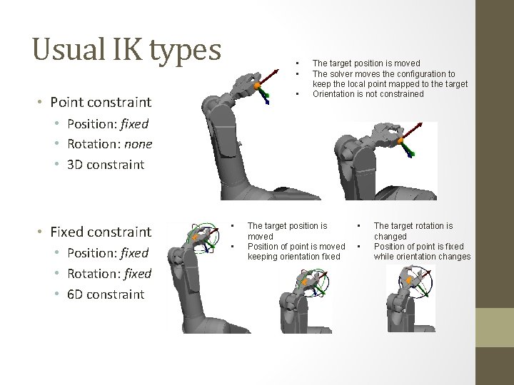
Usual IK types • • Point constraint The target position is moved The solver moves the configuration to keep the local point mapped to the target Orientation is not constrained • Position: fixed • Rotation: none • 3 D constraint • Fixed constraint • • Position: fixed • Rotation: fixed • 6 D constraint • The target position is moved Position of point is moved keeping orientation fixed • • The target rotation is changed Position of point is fixed while orientation changes

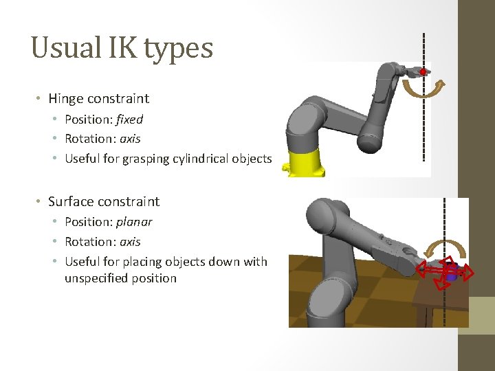
Usual IK types • Hinge constraint • Position: fixed • Rotation: axis • Useful for grasping cylindrical objects • Surface constraint • Position: planar • Rotation: axis • Useful for placing objects down with unspecified position

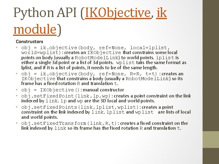
Python API (IKObjective, ik module) Constructors • obj = ik. objective(body, ref=None, local=lplist, world=wplist): creates an IKObjective that constrains some local points on body (usually a Robot. Model. Link) to world points. lplist is either a single 3 d point or a list of 3 d points. wplist taks the same format as lplist, and if it is a list of points, it needs to be of the same length. • obj = ik. objective(body, ref=None, R=R, t=t) : creates an IKObjective that constrains a body (usually a Robot. Model. Link) so its frame has a fixed rotation R and translation t. • obj = IKObjective(): manual constructor • obj. set. Fixed. Point(link, lp, wp): creates a point constraint on the link indexed by link. lp and wp are the 3 D local and world points. • obj. set. Fixed. Points(link, lplist, wplist): creates a point constraint on the link indexed by link. lplist and wplist are lists of local and world points. • obj. set. Fixed. Transform(link, R, t): creates a fixed constraint on the link indexed by link so its frame has the fixed rotation R and translation t.

Python API (IKObjective, ik module) Accessors • obj. num[Pos/Rot]Dims(): returns the number of positions of position / orientation constrained (0 -3) • obj. get. Position(): returns a pair (local, world) of the constrained position. For fixed constraints local is the origin [0, 0, 0] and world is the target point. • obj. get. Position. Direction(): if the position has a planar constraint (num. Pos. Dims()=1), the normal direction of the plane. If this is an linear constraint (num. Pos. Dims()=2), the direction of the line • obj. get. Rotation(): if the rotation is fixed (num. Rot. Dims()=3), the rotation matrix R. • obj. get. Rotation. Axis(): if the rotation is axial (num. Rot. Dims()=2) returns a pair (laxis, waxis) giving the local / world coordinates of the constrained axis. • obj. get. Transform(): if this is a fixed constraint, returns the pair (R, t) giving the fixed transform of the link

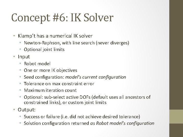
Concept #6: IK Solver • Klamp’t has a numerical IK solver • Newton-Raphson, with line search (never diverges) • Optional joint limits • Input • • • Robot model One or more IK objectives Seed configuration: model’s current configuration Tolerance on max constraint error Maximum iteration count Optional: sub-select active DOFs (default uses all ancestors of constrained links), or custom joint limits • Output: • Success or failure (i. e. did not achieve desired tolerance) • Solution configuration returned as Robot model’s configuration

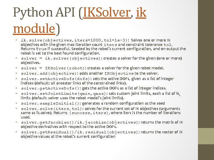
Python API (IKSolver, ik module) • ik. solve(objectives, iters=1000, tol=1 e-3): Solves one or more IK objectives with the given max iteration count iters and constraint tolerance tol. Returns True if successful. Seeded by the robot’s current configuration, and on output the robot is set to the best found configuration. • solver = ik. solver(objectives): creates a solver for the given (one or more) objectives. • solver = IKSolver(robot): creates a solver for the given robot model. • solver. add(objective): adds another IKObjective to the solver. • solver. set. Active. Dofs(dofs): sets the active DOFs, given as a list of integer indices (default: all ancestor links of the constrained links). • solver. get. Active. Dofs(): gets the active DOFs as a list of integer indices. • solver. set. Joint. Limits(qmin, qmax): sets custom joint limits, each a list of NL limits (default: solver uses the robot model’s joint limits). • solver. sample. Initial(): generates a random configuration as the seed • solver. solve(iters, tol): solves for the current set of IK objectives (arguments same as ik. solve). Returns (success, iters), where iters is the number of iterations used. • solver. get. Jacobian()/ik. jacobian(objectives): returns the matrix of IK objective derivatives with respect to the active DOFs. • solver. get. Residual()/ik. residual(objectives): returns the vector of IK objective values at the robot’s current configuration

Example • Find a configuration where the end effector of a planar 3 R robot touches the point (1. 5, 1)

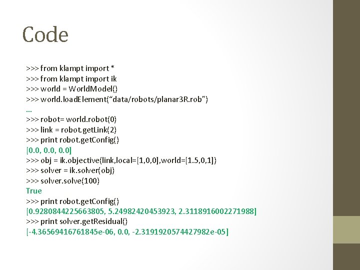
Code >>> from klampt import * >>> from klampt import ik >>> world = World. Model() >>> world. load. Element(“data/robots/planar 3 R. rob") … >>> robot= world. robot(0) >>> link = robot. get. Link(2) >>> print robot. get. Config() [0. 0, 0. 0] >>> obj = ik. objective(link, local=[1, 0, 0], world=[1. 5, 0, 1]) >>> solver = ik. solver(obj) >>> solver. solve(100) True >>> print robot. get. Config() [0. 9280844225663805, 5. 24982420453923, 2. 3118916002271988] >>> print solver. get. Residual() [-4. 36569416761845 e-06, 0. 0, -2. 3191920574427982 e-05]

Code >>> obj 2 = ik. objective(link, local=[1, 0, 0], world=[3, 0, 1. 5]) >>> solver = ik. solver(obj 2) >>> solver. solve(100) (False, 6) >>> print robot. get. Config() [0. 43734637942594445, 0. 0047157337713716885, 6. 278796895032342] >>> print solver. get. Residual() [-0. 2845097603140254, 0. 0, -0. 22482504933765957] >>> print robot. get. Link(2). get. World. Position([1, 0, 0]) [2. 7154902396859746, 0. 0, 1. 2751749506623404] >>> print solver. get. Jacobian() [[-1. 2751749506623402, -0. 8516378500751175, 0. 423833591599536], [0. 0, 0. 0], [2. 7154902396859737, 1. 809611481558724, 0. 9057400767504095]]

Klamp’t TODO • More advanced planning functionality (goal sets, optimization functions, planner diagnosis) • Unified app with built-in world design / planning / optimization / simulation • Massive parallel simulation • Visualizer customization in GUI • Tighter integration with Jupyter Notebooks (saving state, simulations, movies, interactive clicking) • Developers wanted

Next time • Movement along trajectories • Reading: • RS Chapter 15. 1 -2

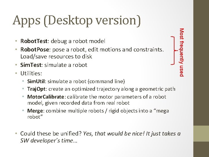
Apps (Desktop version) Most frequently used • Robot. Test: debug a robot model • Robot. Pose: pose a robot, edit motions and constraints. Load/save resources to disk • Sim. Test: simulate a robot • Utilities: • Sim. Util: simulate a robot (command line) • Traj. Opt: create an optimized trajectory along a geometric path • Motor. Calibrate: calibrate the motor parameters of a robot model, given recorded data from real robot • Merge: combine multiple robots / rigid objects into a “mega robot” • Could these be unified? Yes, that would be nice! It just takes a SW developer’s time…

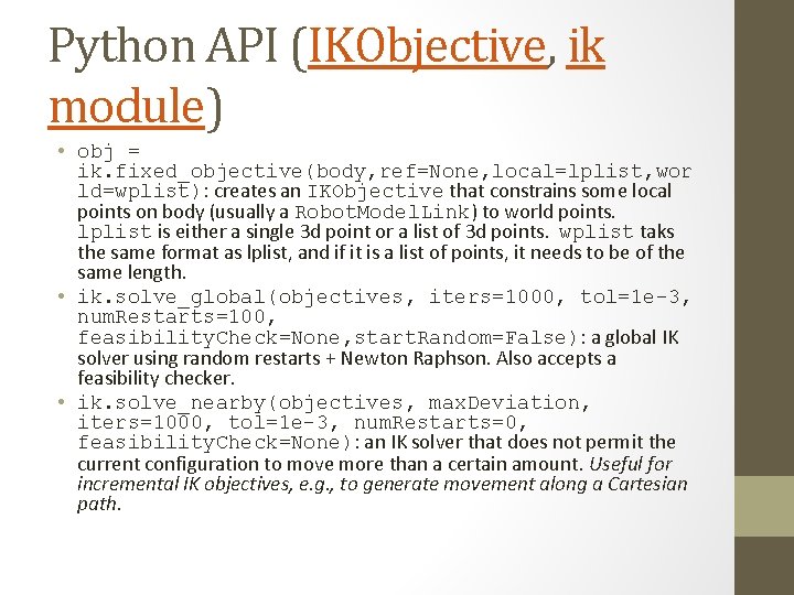
Python API (IKObjective, ik module) • obj = ik. fixed_objective(body, ref=None, local=lplist, wor ld=wplist): creates an IKObjective that constrains some local points on body (usually a Robot. Model. Link) to world points. lplist is either a single 3 d point or a list of 3 d points. wplist taks the same format as lplist, and if it is a list of points, it needs to be of the same length. • ik. solve_global(objectives, iters=1000, tol=1 e-3, num. Restarts=100, feasibility. Check=None, start. Random=False): a global IK solver using random restarts + Newton Raphson. Also accepts a feasibility checker. • ik. solve_nearby(objectives, max. Deviation, iters=1000, tol=1 e-3, num. Restarts=0, feasibility. Check=None): an IK solver that does not permit the current configuration to move more than a certain amount. Useful for incremental IK objectives, e. g. , to generate movement along a Cartesian path.