Introduction to Integration Methods Types of Methods causal

Introduction to Integration Methods

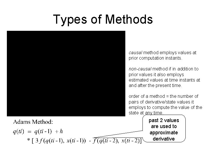
Types of Methods causal method employs values at prior computation instants. non-causal method if in addition to prior values it also employs estimated values at time instants at and after the present time. order of a method = the number of pairs of derivative/state values it employs to compute the value of the state at any time. past 2 values are used to approximate derivative

Causal Methods • A causal method of order m is often a linear combination of the state and derivative values at time instants ti-m to ti-1 with coefficients chosen to minimize the error from the computed estimate to the real value. • Usually the basis of the derivation of the coefficients is the assumption that the state trajectories and the output trajectories are smooth enough to be approximated by the mth order polynomial. • Often it is not known beforehand whether the requisite smoothness indeed obtains. • startup is the determination of the state, derivative, and output values for the times t 1 -m to t 1 at the initial simulation time t 1. Use lower order causal or non-causal methods

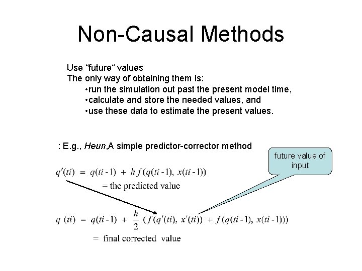
Non-Causal Methods Use “future“ values The only way of obtaining them is: • run the simulation out past the present model time, • calculate and store the needed values, and • use these data to estimate the present values. : E. g. , Heun, A simple predictor-corrector method future value of input

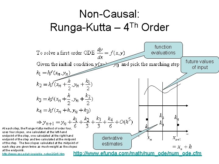
Non-Causal: Runga-Kutta – 4 Th Order function evaluations future values of input At each step, the Runge-Kutta method of order four, uses four slopes, one calculated at the left-hand endpoint of the step, one calculated at the right-hand endpoint of the step and two calculated at the midpoint of the step. The two slopes calculated at the midpoint of each step are given twice as much weight as the slopes at the endpoints. http: //www. gpc. edu/~jcraig/de_notes 2/2 s 6. htm derivative estimates http: //www. efunda. com/math/num_ode. cfm

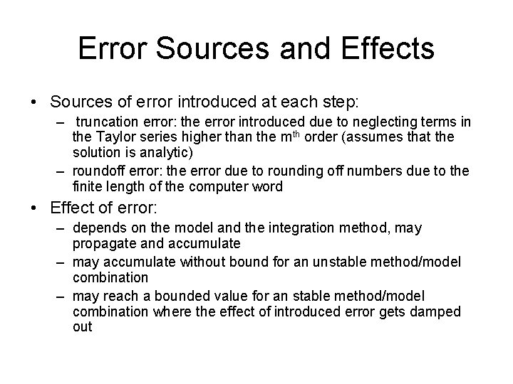
Error Sources and Effects • Sources of error introduced at each step: – truncation error: the error introduced due to neglecting terms in the Taylor series higher than the mth order (assumes that the solution is analytic) – roundoff error: the error due to rounding off numbers due to the finite length of the computer word • Effect of error: – depends on the model and the integration method, may propagate and accumulate – may accumulate without bound for an unstable method/model combination – may reach a bounded value for an stable method/model combination where the effect of introduced error gets damped out

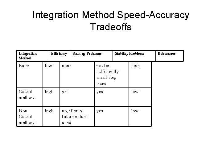
Integration Method Speed-Accuracy Tradeoffs Integration Method Efficiency Start-up Problems Stability Problems Euler low none not for sufficiently small step sizes high Causal methods high yes low Non. Causal methods high no, if only future values used yes low Robustness